How to look at raw and destriped voltage

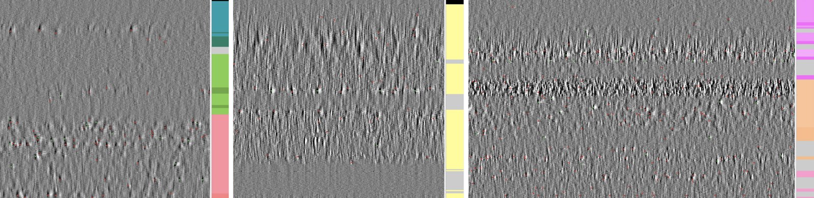
Every feature is computed from a few seconds of voltage. Looking at that voltage first is the quickest check of a recording: whether the probe entered the brain, which channels are dead or noisy, whether destriping behaved. It is also the most direct view of why the atlas works at all: different brain regions look different.

40 ms of destriped AP-band voltage (channels × time) on three probes, with each probe’s brain regions on its right in Allen atlas colours. Firing density and spike size change from region to region, in the same voltage.

A destriped snippet

get_destriped_snippet reads one window and runs the same destriping as feature computation, without computing any feature. See tune the computation for its fields:

figure_voltage_snippets draws each one as an image, channels × time:

import ephysatlas.plots
from ephysatlas.feature_calculators import SnippetWindow, SpikeGLXFileFeatureCalculator

calc = SpikeGLXFileFeatureCalculator(
    ap_file="/data/probe00.ap.cbin", lf_file="/data/probe00.lf.cbin"
)
snippet = calc.get_destriped_snippet(
    SnippetWindow(t_start=300.0, duration_ap=1.0, duration_lf=1.0)
)
fs_ap, fs_lf = snippet.raw.fs_ap, snippet.raw.fs_lf

fig, axs = ephysatlas.plots.figure_voltage_snippets({
    "AP band, destriped": (snippet.des_ap[:, : int(0.05 * fs_ap)], fs_ap),  # 50 ms shows single spikes
    "LF band, destriped": (snippet.des_lf, fs_lf),  # the LF needs the whole second
})

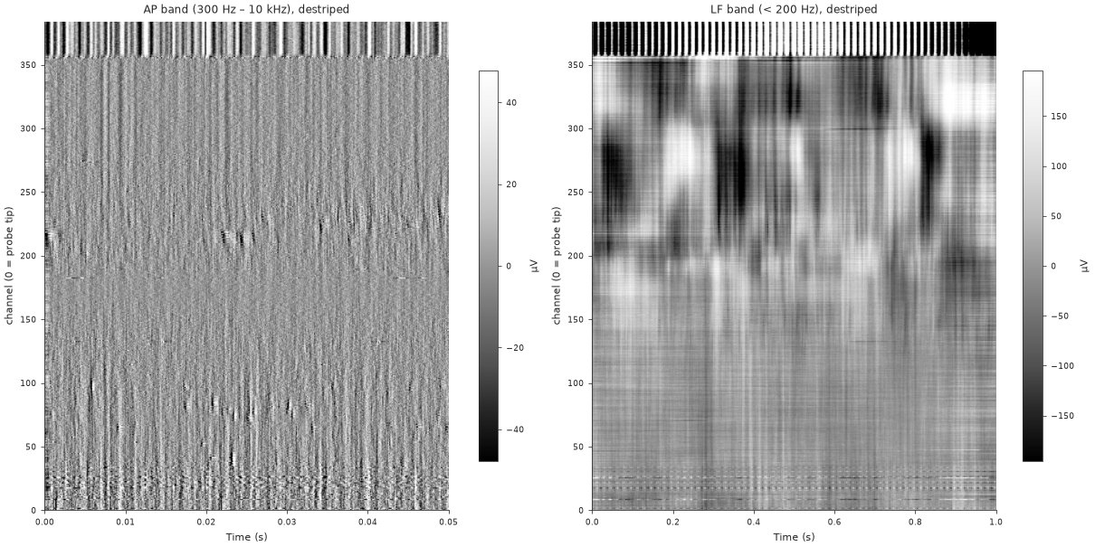
1 s of destriped voltage committed in this repository (tests/fixtures/ap_destriped.npy, lf_destriped.npy), drawn by the code above. The top ~25 channels carry a large, regular artefact rather than brain signal, as channels outside the brain often do.

By default each panel’s colour range is ±4 times its median channel standard deviation: set on the typical channel rather than on the extremes, because the channels outside the brain are many times larger and would grey out everything else. Pass vrange (in µV) to use one range for every panel. show_colorbar and show_titles turn those parts off. examples/plot_voltage_snippets.py draws this figure from the committed snippet.

Raw against destriped

Neuropixels voltage carries artefacts shared across channels: common-mode noise, and stripes from the multiplexed ADCs that sample channel groups at slightly different times. Destriping removes them before any feature is computed. It is ibldsp.voltage.destripe (AP) and destripe_lfp (LF) from ibl-neuropixel, called through ephysatlas.feature_computation.destripe_ap_lf.

The same 10 ms of AP voltage after a high-pass filter only (A), after also subtracting the median across channels (B), and after full destriping (C), which also corrects the sampling-time shift of each channel and filters spatially. Only C leaves the spikes on a flat background.

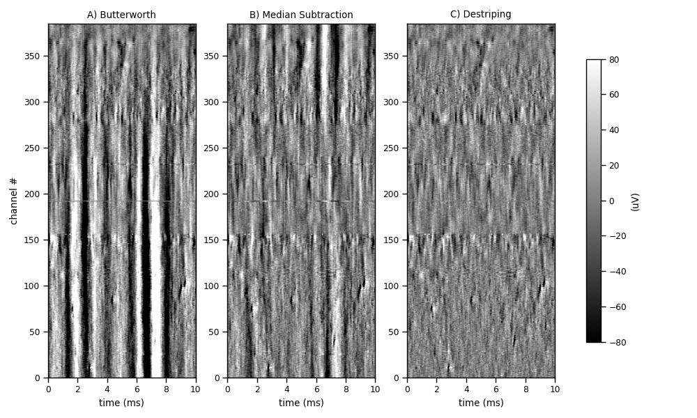
To check the destriping of your own recording, draw the raw AP beside the destriped AP (or the LF pair) with the same function:

n = int(0.05 * fs_ap)   # 50 ms
fig, axs = ephysatlas.plots.figure_voltage_snippets({
    "AP, raw": (snippet.raw.raw_ap[:, :n], fs_ap),
    "AP, destriped": (snippet.des_ap[:, :n], fs_ap),
})

get_destriped_snippet takes a DestripeOptions to try other destriping settings on the inspection alone.

Bad channels

Destriping needs to know which channels to leave out. Each channel is labelled from the raw AP band: 0 good, 1 dead, 2 noisy, 3 outside the brain. The labels travel on as the channel_labels feature column, and outside is derived from them.

ibldsp’s bad-channel detection on raw AP: (a) similarity to the neighbouring channels, low for a dead channel; (b) high-frequency power, high for a noisy one; (c) the trend of the similarity along the probe, which drops past the brain surface. Red marks are the flagged channels, dashed lines the thresholds; (d) is 100 ms of the raw voltage.

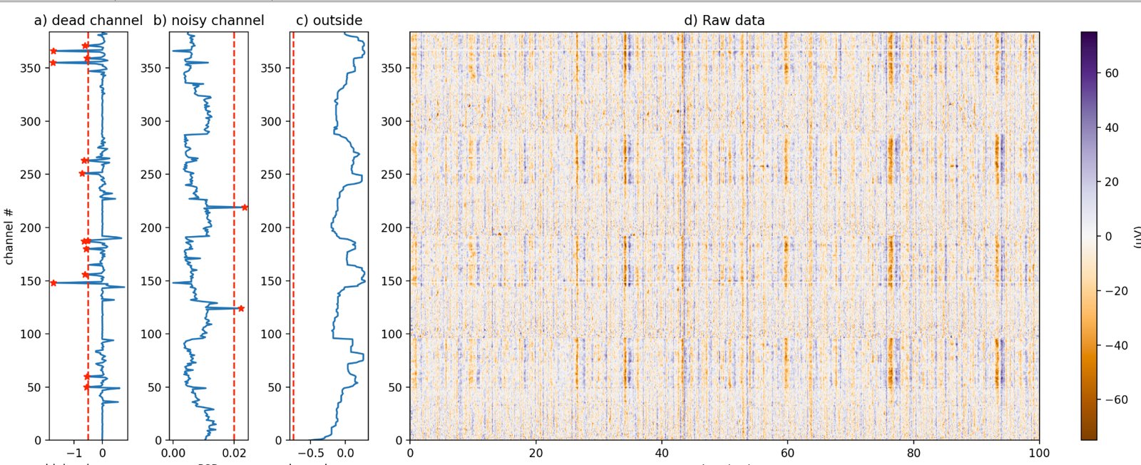
The same figure for your own recording is one call:

import numpy as np
from ibldsp.voltage import detect_bad_channels

labels, xfeats = detect_bad_channels(
    snippet.raw.raw_ap, fs=snippet.raw.fs_ap, display=True
)
print(np.bincount(labels.astype(int), minlength=4))   # good, dead, noisy, outside

snippet.channel_labels holds the labels feature computation actually used: those of the channel table when the source has one, detected from the snippet otherwise.

For IBL insertions

ephysatlas.reveal.AtlasReveal draws these views for any IBL probe insertion, given ONE access: figure_04_ap_voltage (raw and destriped AP), figure_05_lfp_voltage (LF and its current-source density) and figure_06_bad_channels.

from one.api import ONE
from ephysatlas.reveal import AtlasReveal

reveal = AtlasReveal(one=ONE(), pid="0228bcfd-632e-49bd-acd4-c334cf9213e9")
reveal.figure_04_ap_voltage()

The IBL documentation shows how to load raw ephys data of any public insertion yourself.

Next steps

• Compute features from the recording you just checked
• The feature pipeline — what happens after destriping
• Features along the probe — the features this voltage turns into