How to load encoding volumes
This guide downloads and loads encoding volumes — a pre-computed 4-D volumetric representation of electrophysiological features on the Allen Common Coordinate Framework (CCF). Where the channel features are a table of measured channels, an encoding volume is the features projected onto a regular voxel grid covering the whole brain.
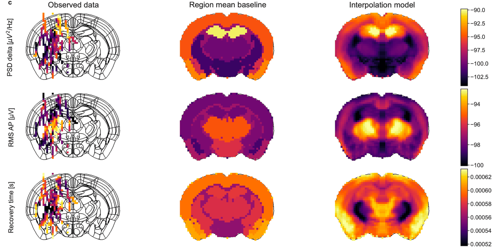
To browse the volumes without downloading them, use the IBL Ephys Atlas viewer. To draw them on atlas slices, see atlas maps.
These volumes are in a private S3 bucket and need an IBL account — pass a logged-in one.api.ONE instance.
S3 layout
aggregates/atlas/encoding_volumes/{project}/{label}/
├── brainwide_ephys_atlas_{res_um}um.npz   4-D volume (nx, ny, nz, N_features)
└── brainwide_ephys_edges_{res_um}um.npz   ephys edges (nx, ny, nz, 1)
Encoding volumes are versioned along two independent axes: the vintage label (label) and the voxel resolution (res_um, in µm). A 25 µm volume is roughly (456, 528, 320) and ~500 MB; a 50 µm volume is (228, 264, 160) — 138 MB for 2026_W42, which is published at 50 µm only.
Which vintages and resolutions exist changes as new ones are published. List them rather than assuming:
import ephysatlas.data

labels = ephysatlas.data.list_available_labels(one=one, project="ea_active")
Download
from pathlib import Path

import numpy as np
from one.api import ONE
from ephysatlas.data import download_encoding_volume

one = ONE()
local_path = Path("/datadisk/ephys-atlas/volumes")

# res_um omitted -> auto-resolves to the finest resolution available for this label
file_path = download_encoding_volume(local_path, label="2026_W42", one=one)

data = np.load(file_path, allow_pickle=True)
label defaults to "2026_W42". Pass res_um (in µm) to choose a resolution instead of the finest one available.
What the file contains
N is the number of features: 43 for 2026_W42. The set has the spike-shape columns (spike_width_secs, …) instead of the raw waveform ones (peak_val, …), the multi-channel spatial_spread_um and slowness_s_per_m, and the first spatial differences *_bpr.
| key | shape | dtype | description |
|---|---|---|---|
ephys_atlas_vol |
(nx, ny, nz, N) |
float16 | The 4-D volume: x × y × z × features, i.e. ML × AP × DV |
feature_names |
(N,) |
str | Feature name strings, ordered as the last axis |
mean_per_feature |
(N,) |
float32 | Per-feature normalisation mean |
std_per_feature |
(N,) |
float32 | Per-feature normalisation standard deviation |
grid_shape |
(3,) |
int32 | Volume grid dimensions [nx, ny, nz] |
res_um |
(1,) |
int32 | Voxel resolution, µm |
Extract one feature’s volume
Always look the feature up by name — the ordering of the last axis is not guaranteed stable across vintages:
vol = data["ephys_atlas_vol"]
feature_names = data["feature_names"]

idx = np.where(feature_names == "rms_ap")[0][0]
rms_ap_volume = vol[..., idx]   # (nx, ny, nz) float16
The axis order is ML × AP × DV. iblatlas atlases use AP × ML × DV, so transpose the first two axes (np.transpose(vol, (1, 0, 2, 3))) before indexing a volume with atlas coordinates.
Units and normalisation
Values are stored in raw, unnormalised feature units, with 0.0 outside the brain mask.
mean_per_feature and std_per_feature are provided for optional z-scoring and are not pre-applied. To z-score:
z = (vol[..., idx] - data["mean_per_feature"][idx]) / data["std_per_feature"][idx]0.0 outside the brain mask is indistinguishable from a genuine zero measurement. Build a mask from a feature that is never legitimately zero inside the brain (rms_lf, say) before computing any statistic over the volume, or the out-of-brain voxels will drag every mean towards zero.
Ephys edges
An encoding volume says what the ephys signature is at each voxel. Its edges say where that signature changes fastest — boundaries between electrophysiologically distinct territories, found from the features alone.
The published edges sit next to the volume on S3. download_edges_volume takes the same arguments as download_encoding_volume:
from ephysatlas.data import download_edges_volume

edges_file = download_edges_volume(local_path, label="2026_W42", one=one)
edges = np.load(edges_file)["ephys_atlas_vol"][..., 0]   # (ML, AP, DV) float16, 0 outside the mask
The file has the encoding volume’s layout, so it reads the same way: a single feature, feature_names = ["ephys_edges"], 6 MB at 50 µm.
Derive them yourself
To recompute the edges, or derive them with other settings:
from ephysatlas.edges import compute_edges_volume

edges = compute_edges_volume(file_path)   # (AP, ML, DV) float32, NaN outside the mask
The volume is z-scored and rotated onto its principal components. The components that explain 95 % of the variance are kept and whitened, so Euclidean distance between voxels is their Mahalanobis distance in feature space; 2026_W42 keeps 7. Each component is Gaussian-smoothed (σ = 100 µm, NaN-aware) and its gradient magnitude taken, per mm. The magnitudes are then aggregated across components:
aggregate |
units |
|---|---|
"median" (default) |
median across PCs of the whitened PC gradient magnitude, per mm — robust to a PC that changes alone |
"mean" |
mean across PCs, per mm |
Voxels within 100 µm of the mask border are dropped (erode_um), because their gradient is a mask artefact. void and void_fluid are excluded; root is kept, as it contains fibre tracts. The mask comes from iblatlas.atlas.AllenAtlas(res_um) unless you pass atlas=, and that atlas downloads its Allen volumes on first use.
compute_edges_volume also writes brainwide_ephys_edges_{res_um}um.npz next to the volume (or to out_file=), in the layout published on S3:
| key | content |
|---|---|
ephys_atlas_vol |
(ML, AP, DV, 1) float16 edge strength, e.g. (228, 264, 160, 1) at 50 µm; 0 outside the eroded mask |
feature_names |
["ephys_edges"] |
res_um, grid_shape |
As in the encoding volume |
axis_order |
"ML,AP,DV" |
units |
The aggregate’s units, as in the table above |
aggregate, sigma_um, erode_um, n_pcs, variance_threshold, exclude_acronyms, source |
The settings used, for the record |
On the 2026_W42 volume this takes about 5 seconds and reproduces the published file exactly; 61 % of the grid is outside the eroded brain mask (NaN), and the median edge strength is 1.6 per mm.
For other settings, the steps are separate functions: load_whitened_pcs (whitened PCs and the valid mask), edge_strength (smoothed gradient, aggregated) and save_edges_volume (write in the encoding volume’s layout). See the edges API.
Next steps
- Atlas maps — plot a volume on atlas slices
- Load channel features — the tabular source these volumes are built from
- Predict features from position — the spatial encoder answers a similar question with a model rather than a lookup
- S3 layout reference
download_encoding_volumeAPI,download_edges_volumeAPI andcompute_edges_volumeAPI