The feature pipeline
What happens between raw voltage and a row in a feature table, and why the steps are arranged the way they are.
The path
   your recording
        │
        │  a calculator normalises the source
        ▼
   raw AP / LF arrays  (n_channels, n_samples), volts  +  geometry  +  channel labels
        │
        │  destripe_ap_lf  —  the single shared destriping primitive
        ▼
   destriped AP / LF
        │
        │  features.lf / .csd / .ap / .spikes
        ▼
   per-snippet feature tables      <feature>_features.pqt
        │
        │  aggregation             median across snippets
        ▼
   raw_ephys_features.pqt
        │
        │  denoising               per-probe outlier suppression + transforms
        │  waveform remap          raw waveform columns -> spike-shape columns
        ▼
   raw_ephys_features_denoised.pqt        ← what models consume
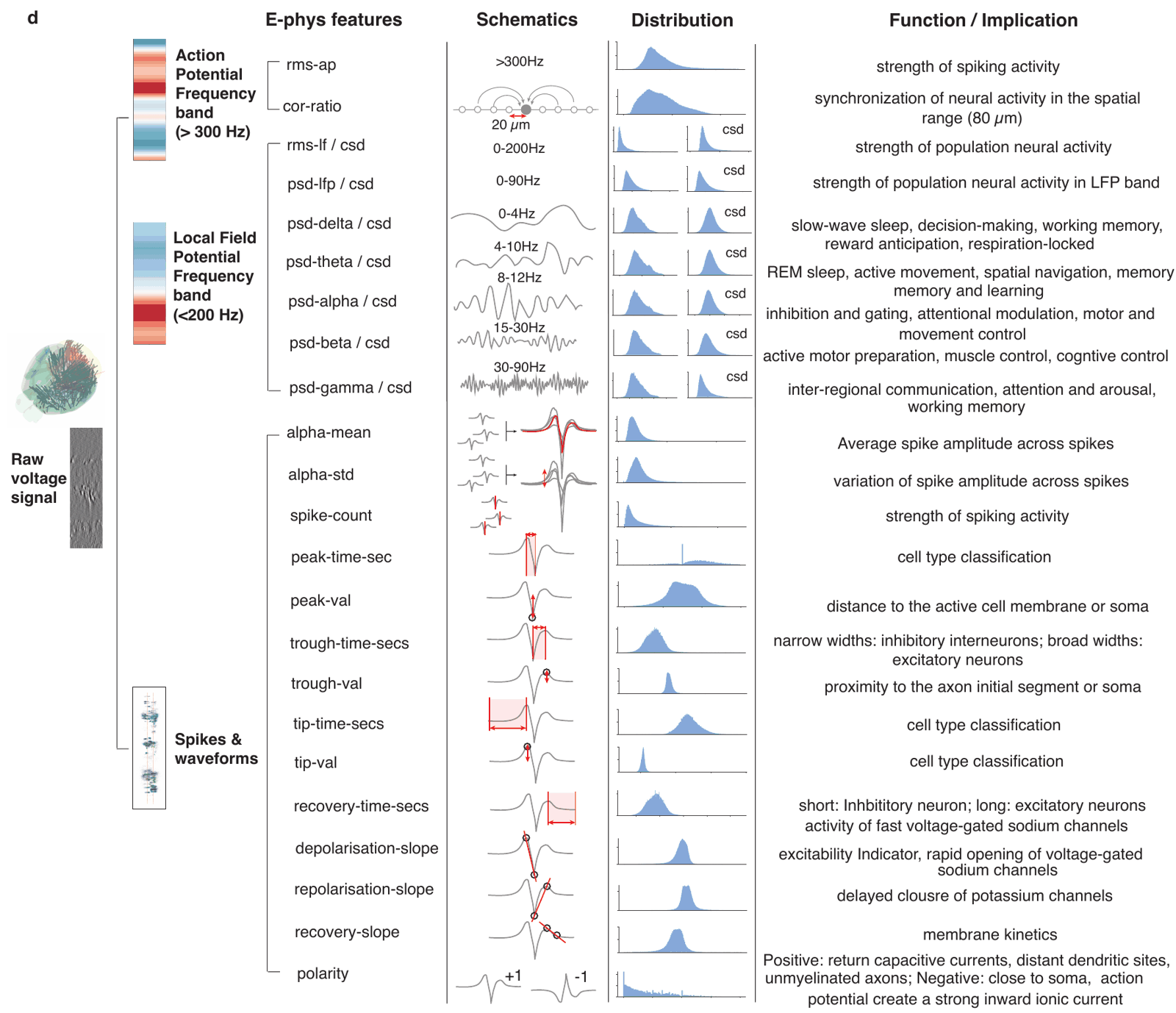
What the features are, band by band:
One source interface, many formats
The first design decision: normalise the source, then share everything downstream.
Every calculator subclasses BaseFeatureCalculator and implements only how to obtain raw arrays and channel metadata. Once a recording is (n_channels, n_samples) in volts plus a geometry dict, nothing further cares whether it came from SpikeGLX, NWB, Zarr, an lfpack archive or an array in memory.
BaseFeatureCalculator                      abstract source interface + compute_snippet
├── SpikeGlxLikeFeatureCalculator          shared spikeglx.Reader contract
│   ├── SpikeGLXFileFeatureCalculator      local AP/LF .bin/.cbin
│   └── IBLPIDFeatureCalculator            IBL insertion via ONE
├── SpikeInterfaceFeatureCalculator        shared SI BaseRecording contract
│   ├── NwbFeatureCalculator               NWB: local, streamed, DANDI
│   └── SpikeInterfaceZarrFeatureCalculator SI-native Zarr
├── LFPackFeatureCalculator                LF only: an lfpack archive
└── NumpyArrayFeatureCalculator            LF only: an array in memory
The two intermediate classes exist because reader-contract logic — reading a snippet, filling geometry defaults, resolving channel labels — is identical within each family and would otherwise be duplicated per source.
As a result, supporting a new format needs little code: implement _open_reader or _open_recording and all the feature computation then works for it. A source with no reader to share implements load_raw_snippet directly, as the two LF-only calculators do. Every calculator also inherits compute_denoised_features, the multi-snippet route.
Composition for the acquisition axis
NwbFeatureCalculator faces a second problem: an NWB recording varies by backend (HDF5 or Zarr) and by location (local, URL, DANDI). Four combinations, and subclassing would give four classes.
Instead both axes are fields on one value object, NwbSource, and the calculator holds one source per band. The combinatorial axis became data instead of types.
Destriping is shared with the debug path
Neuropixels raw voltage carries structured artefacts — common-mode noise, per-channel offsets, ADC striping. Destriping removes them before any feature is computed.
destripe_ap_lf delegates to ibldsp.voltage.destripe (AP) and ibldsp.voltage.destripe_lfp (LF), from ibl-neuropixel. Both compute_features_from_raw and get_destriped_snippet call it, so the features and the voltage you plot come from the same code.
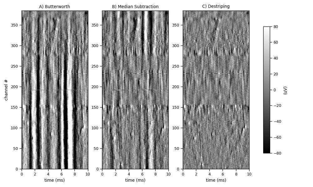
get_destriped_snippet is the inspection path — what you use to check whether destriping is behaving. If it had its own copy of the logic, it could drift from the production path and you would be debugging a different pipeline than the one producing your features.
Bad channels are handled here rather than dropped. channel_labels marks each channel good, dead, noisy, or outside the brain, and destriping interpolates over the bad ones. The labels then travel forward as a feature column, so a model can learn to distrust them rather than having to guess. How the labels are decided: bad channels.
LF that arrives already preprocessed — an lfpack archive, a decimated array — skips this step with FeatureComputationOptions(skip_lf_destripe=True): destriping it again at its decimated sample rate would fail. With destriping skipped, the channel labels come from the source’s channel table instead.
Feature families, and why they are separate
Four families, computed independently:
| family | band | measures |
|---|---|---|
lf |
LF | Band power, RMS, spectral decay |
csd |
LF | The same, on the current-source density and the bipolar reference |
ap |
AP | AP-band RMS, channel cross-correlation |
waveforms |
AP | Spike detection and waveform shape |
They are separate because their costs differ by orders of magnitude. lf and csd are spectral estimates on a decimated signal — seconds. waveforms runs DARTsort spike detection over the AP band — minutes to hours, and a heavy dependency tree that only ships in the [full] extra.
Being separable means you can compute the cheap families on everything and the expensive ones only where needed. It is also why each family writes its own <family>_features.pqt: skip_saved_computation can then reuse a completed family and recompute only what is missing, making a long run resumable.
Why CSD as well as LF
The LFP at a channel is a mixture of activity from a wide radius — volume conduction is not local. The current-source density, a spatial second derivative across channels, is far more local, so psd_delta and psd_delta_csd carry different information about the same signal. Both go in, and the decoder uses both. The *_bpr columns sit in between: the first spatial difference, a bipolar reference between neighbouring contacts.
Spatial derivatives amplify noise, so the LF is Cadzow-denoised first. The parameters depend on the layout (features.cadzow_lfp_kwargs): the NP1 checkerboard is filled onto its full lateral × depth grid, which removes the seams the spatial windows used to leave in the CSD, while NP2 contacts already fill theirs.
Snippets, and why several
A snippet is one time window. The SnippetWindow defaults — duration_ap=5.0, duration_lf=25.0 — reflect a difference between the bands: LF features need a long window to resolve low-frequency power, while AP features are expensive and converge quickly.
But per-channel estimates from a single window are noisy. Compute several windows spread through the recording and take their median, and the estimates stabilise. This is what the training data did, which is why matching it matters for inference.
calc.compute_denoised_features(n_snippets=...) does exactly that. It leaves out the first and last 5 minutes, draws one start time (in whole seconds) in each of n_snippets equal stretches of the rest, computes every snippet, then aggregates and denoises. get_snippet_start_times and compute_aggregated_features expose the two halves, to choose the windows yourself.
The output layout follows from that. The snippet directory name encodes t_start, duration_ap and duration_lf, so windows over the same recording sit side by side and never collide:
<name>/
├── channels.pqt                                    per-probe, written once
├── probe_<name>_000300.0_01.0_01.0/
└── probe_<name>_000900.0_01.0_01.0/
channels.pqt sits at the probe level because geometry and anatomy are properties of the insertion, not of a time window.
Merging on physical position, not channel number
Channel metadata is merged onto the feature table on the physical recording site — (axial_um, lateral_um, shank), rounded to the nearest micrometre — not on the channel index.
Version 0.7.0 made this change. Channel numbering is unreliable across data sources: rawInd, the SpikeGLX index and the SpikeInterface index do not agree in general, so joining on a channel number can attach anatomy to the wrong channel without any error. Physical position is unambiguous. rawInd is still carried, as descriptive metadata only.
One shank per calculator
Feature computation assumes all channels of a calculator are on one shank. Several steps work on the x / y positions (or the channel order) alone, and on a multi-shank probe those do not tell the shanks apart: x is measured within each shank. On a four-shank Neuropixels 2.0 probe (NP2.4), all four shanks report the same x (27–59 µm) and the same columns, so the 384 channels sit on only 96 distinct (x, y) positions.
| step | uses | on a multi-shank probe |
|---|---|---|
Destriping (ibldsp destripe, destripe_lfp) |
geometry["shank"] |
Shank-aware: CAR and the k-filter run per shank. Bad-channel interpolation uses x / y only |
| Channel metadata merge | (axial_um, lateral_um, shank) |
Shank-aware |
lf family |
each channel alone | Unaffected beyond destriping |
csd family (Cadzow, then current_source_density) |
x / y, col, row |
On a synthetic four-shank recording the default raises ZeroDivisionError in ibldsp.cadzow.cadzow_denoiser. With CsdParams(denoise=False) the zero spacing between shanks gives NaN, and the schema check raises SchemaError. Only with scale=False as well does it run, and then channels of different shanks at the same depth are differenced against each other |
cor_ratio in the ap family (xcor_acor_ratio) |
the 8 neighbouring channel numbers either side | Neighbours can lie on another shank — no error |
waveforms (DARTsort) |
x / y only |
The shanks overlap in DARTsort’s view of the probe, so detection neighbourhoods and spike localisation mix them — no check |
Denoising at aggregation (EphysDenoiser) |
(lateral_um, axial_um) |
Every shank is put on one grid and filtered as a single surface — no error |
Only the NWB and Zarr calculators check. A recording whose SpikeInterface channel groups span more than one shank raises:
NotImplementedError: <name>: recording spans 4 shanks/groups ([0, 1, 2, 3]); per-shank
feature computation is not implemented yet. Pass a single shank's channels per calculator
(one ElectricalSeries per shank, or a per-shank channel subset).
The SpikeGLX and IBL PID calculators do not check, and the LFPack and NumPy calculators set shank to 0 when the geometry has none.
So compute one shank at a time. For the LF families, slice each shank’s channels and geometry into its own NumpyArrayFeatureCalculator; each shank then gets its own pid and a correct shank column:
import numpy as np
import neuropixel

from ephysatlas.feature_calculators import (
    FeatureComputationOptions,
    NumpyArrayFeatureCalculator,
    SnippetWindow,
)

h = neuropixel.trace_header(version=2, nshank=4)   # or your recording's geometry
# lf: (384, n_samples) LF in volts, at its native rate fs_lf

for shank in np.unique(h["shank"]):
    sel = h["shank"] == shank
    calc = NumpyArrayFeatureCalculator(
        lf=lf[sel],
        fs_lf=fs_lf,
        geometry={key: np.asarray(value)[sel] for key, value in h.items()},
        name=f"my_probe_shank{int(shank)}",
    )
    result = calc.compute_snippet(
        SnippetWindow(t_start=0.0, duration_ap=1.0, duration_lf=25.0),
        FeatureComputationOptions(features_to_compute=["lf", "csd"], include_trajectory=False),
    )
On the same synthetic four-shank recording, each shank computed this way gets the NP2 Cadzow defaults and gives finite lf and csd features. There is no per-shank route yet for the AP families (ap, waveforms) from a SpikeGLX file.
Aggregation and denoising
Three steps, all per-probe.
Aggregation reduces the per-snippet tables to one row per (pid, channel): the median of each feature across snippets, except spike_count, whose mean counts a snippet with no spikes as zero.
Denoising is two operations in sequence, EphysTransformer then EphysDenoiser:
- Transform. Features whose schema declares one are transformed first —
rms_apandrms_lfto dB,spike_countto log2. Order matters: the filter then runs in log space, which is the right space for quantities that vary multiplicatively across the brain. - Filter. A total-variation (Chambolle) filter over the probe surface. Each feature is interpolated onto a regular grid in
(lateral_um, axial_um), filtered, and interpolated back. Channels with a non-zero label are dropped and interpolated over rather than filtered.
The filter relies on neighbouring sites being 20 µm apart on an NP1 probe and largely sampling the same tissue, so a channel departing sharply from its neighbours is more likely noisy than different. Total variation is used instead of a smoothing filter because it preserves edges, such as region boundaries.
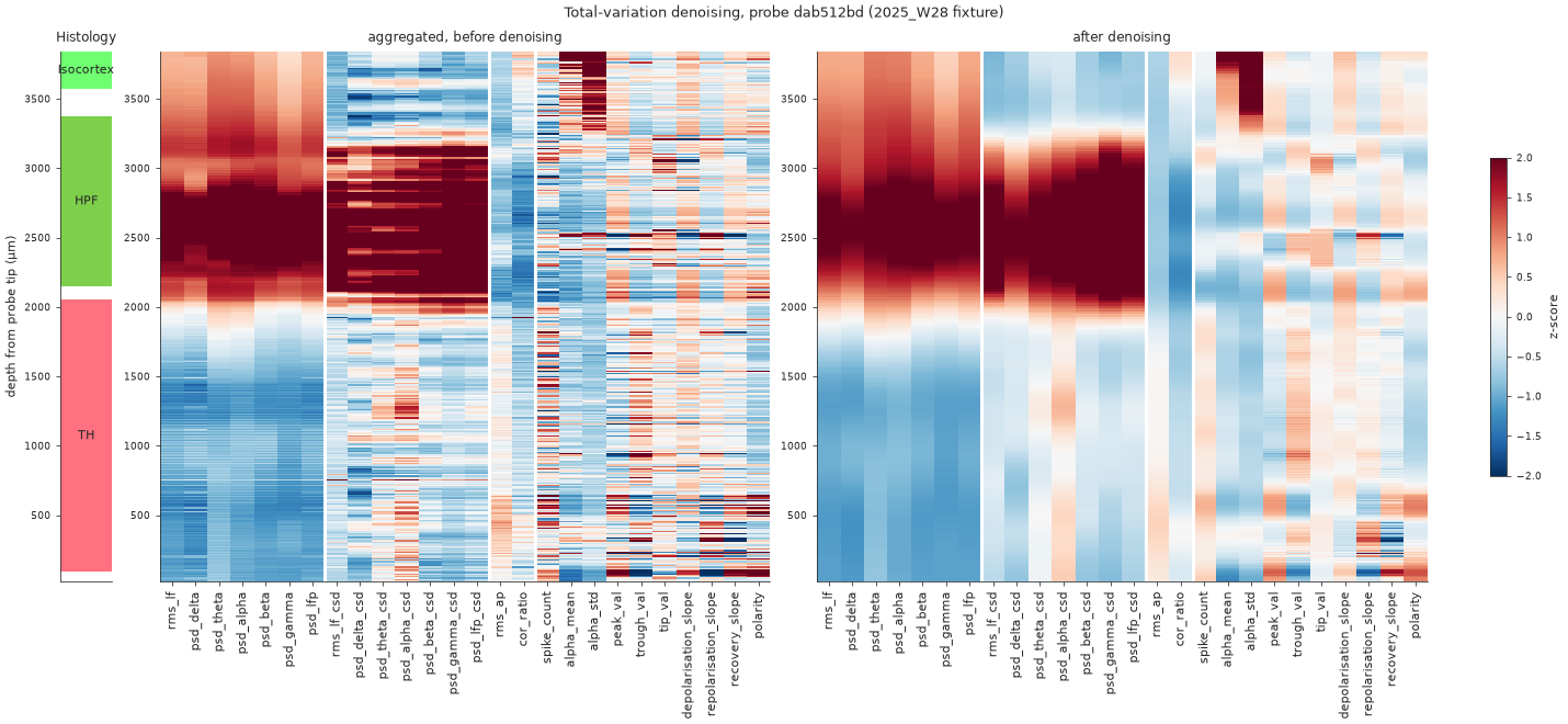
2025_W28 fixture, z-scored, before (left) and after (right) denoising, on one colour scale. The channel-to-channel noise goes; the boundaries at the hippocampus (HPF) and thalamus (TH) stay sharp. Code.fac sets the filter strength in median-deviation units; higher denoises harder. It is set per feature group: DEFAULT_FAC is 0.1 for the AP, LF and CSD groups and 3 for waveforms, chosen by a sweep against region-classification accuracy.
The waveform remap (aggregation.apply_waveform_remap, since 0.9.0) then replaces the six raw timing and amplitude waveform columns with four interpretable spike-shape ones — spike width, pre-depolarisation width, amplitude and peak-to-trough ratio. The six are redundant, and reparametrising them loses no relative information.
That transform and that remap are the reasons the denoised table is not interchangeable with the raw one. See core concepts.
Provenance
Every written feature file carries the package versions and parameters in its pandas .attrs. get_aggregated_snippets_df reads those attrs back to build the snippet table that drives aggregation, so aggregation depends on them. The aggregated table of compute_aggregated_features carries its own: the snippet windows (snippet_windows), the features_version and the ibleatools version and git commit, which pandas keeps when the table is saved to parquet.
When skip_saved_computation reuses a cached family, that file keeps the provenance of the run that created it. A mixed directory therefore records the provenance of each part separately.
Schemas as the contract
Pandera schemas in ephysatlas.features declare every feature column with its dtype, description and unit metadata. ModelRawFeatures is the union of all families; ModelDenoisedFeatures is the same with the spike-shape columns in place of the raw waveform ones.
They are what makes the feature list reference derivable from code rather than hand-maintained, and validation runs at read time (read_features_from_disk(strict=True)) so a malformed table fails at the boundary instead of deep inside a model. The reader picks the schema from the columns the table actually carries, so a denoised table written before the remap still validates.
See also
- Core concepts — vintages, and the raw/denoised distinction
- Compute features from SpikeGLX files
- Tune feature computation
- Feature list