How to map features across the brain
Down one probe, features change at region boundaries. Across the brain they form a map: what a channel at any position should record. ibleatools gives you that map two ways, from the spatial encoder (public) or from the published encoding volumes (IBL account). The IBL Ephys Atlas viewer shows it in the browser.
ephys-atlas.iblcore.org is a browser viewer for the atlas and the brain-wide maps around it: the recorded features, the predicted encoding volumes, gene expression atlases, the lipidome and Brain-Wide Map task responses. All are registered to the Allen atlas, so you can compare them slice by slice. It can also load a compatible dataset of your own, which stays in your browser. Its user guide explains the views.
From sparse recordings to a dense map
The recordings sample the brain sparsely, along probe tracks. The spatial encoder fills the space between them from two sources: the recorded channels nearby, on other probes, and the molecular context at the position (MERFISH cell-type densities and AGEA gene expression from the Allen Institute).

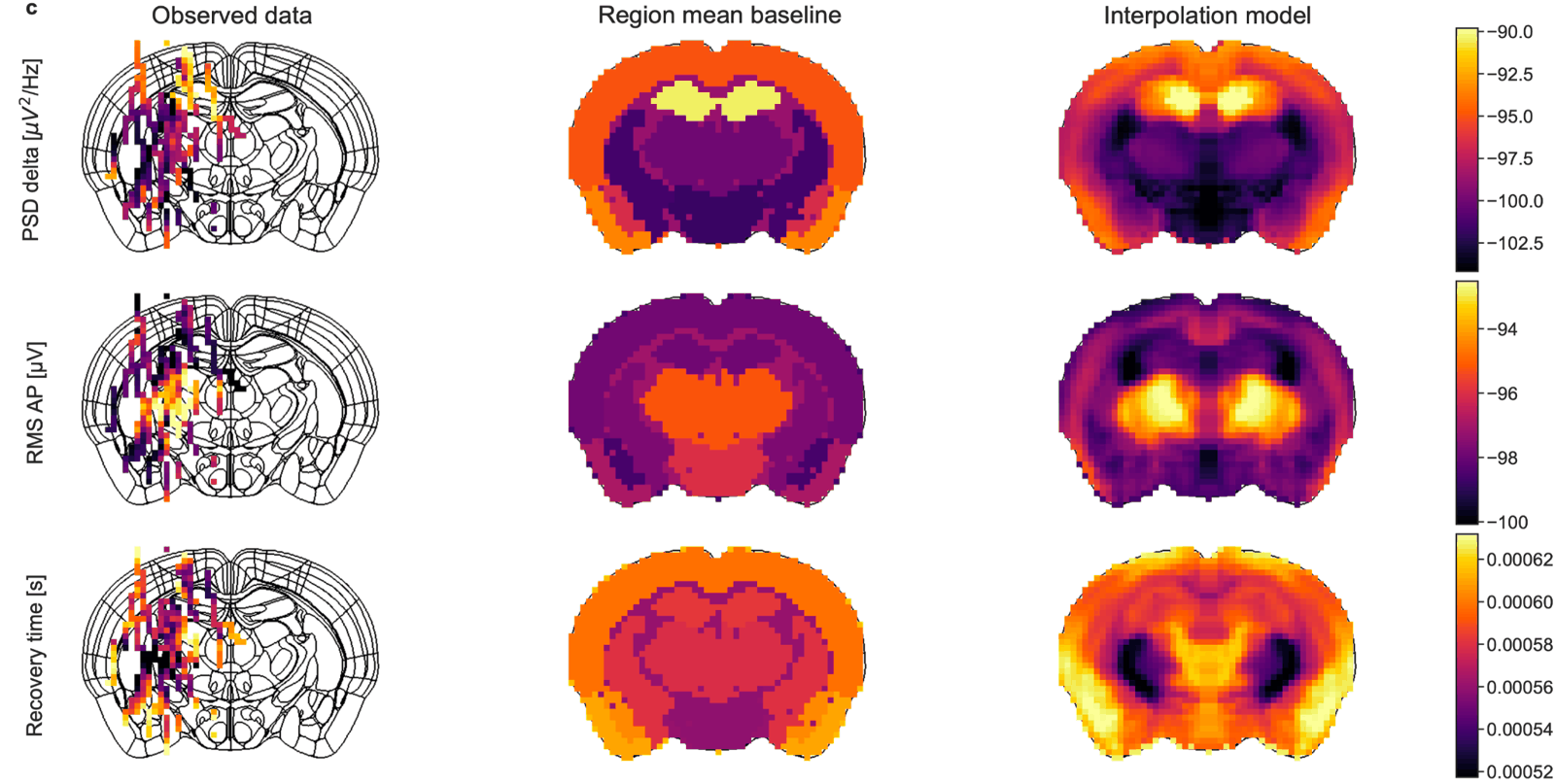
A dense map is more than a per-region average. Within a region the features vary, and the model keeps that variation:
A coronal map from the spatial encoder
No account needed: the encoder is public, and iblatlas provides the brain mask and the region outlines. Predict every voxel of one coronal plane, then draw it:
from iblatlas.atlas import AllenAtlas
import ephysatlas.plots
from ephysatlas import load_pretrained

ba = AllenAtlas(res_um=25)   # downloads the Allen volumes on first use
encoder = load_pretrained("int-brain-lab/ea-encoder-channel", revision="2026_W45")

# Every 4th voxel (100 µm) of the coronal plane at AP = -2 mm, inside the brain
fig, axs = ephysatlas.plots.figure_encoder_coronal(
    encoder,
    ["psd_delta", "rms_ap", "spike_amplitude"],
    ap_m=-2000e-6,                       # metres from bregma
    brain_atlas=ba,
    scales={"spike_amplitude": 1e6},     # volts -> µV
    units={"psd_delta": "dB rel. V²/Hz", "rms_ap": "dB rel. V", "spike_amplitude": "µV"},
)
That is about 6,000 positions, predicted in seconds, in one call to encoder.predict_xyz.
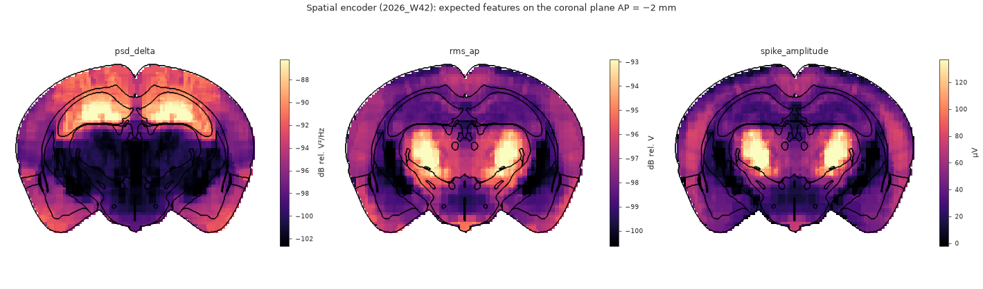
step sets the spacing of the predicted voxels and percentiles the colour range of each panel (2 % to 98 % of its values by default). show_boundaries, show_colorbar and show_titles turn those parts off. examples/plot_encoder_maps.py draws this figure.
Coordinates are in metres, in the IBL bregma-centred space of iblatlas, as everywhere in ibleatools. See predict features from position for the encoder itself, and the IBL notebook working with the atlas for slices and coordinates.
The published encoding volumes
With an IBL account, the encoding volume of each vintage is the same map precomputed on a regular grid, every feature at once. Load encoding volumes covers the download and the file. Its axes are ML × AP × DV; transposed to AP × ML × DV it has exactly the shape of AllenAtlas(res_um), so the iblatlas slice plots take it as is:
import numpy as np
from iblatlas.atlas import AllenAtlas
from iblatlas.plots import plot_volume_on_slice

res_um = int(data["res_um"][0])
idx = np.where(data["feature_names"] == "rms_ap")[0][0]
volume = np.transpose(data["ephys_atlas_vol"][..., idx], (1, 0, 2)).astype(float)
volume[volume == 0] = np.nan                   # 0 is outside the brain mask

plot_volume_on_slice(volume, coord=-2000, slice="coronal", mapping="Cosmos",
                     cmap="magma", brain_atlas=AllenAtlas(res_um=res_um))
coord is in µm here. The ephys edges of a volume, where the signature changes fastest, plot the same way.
For values that are one number per region rather than per voxel, iblatlas also draws region values on slices and on the Swanson flat map.
Next steps
- Predict features from position — the encoder, and comparing it against a recording
- Load encoding volumes — the precomputed maps
- Model families — how the encoder works