Visualise
Every figure the documentation shows, and the page that makes it
Most of what ibleatools computes is best read as a picture: features against depth beside the brain regions, region predictions with their uncertainty, voltage before and after destriping, maps across the brain. Each card below links to the page with the code that draws it.
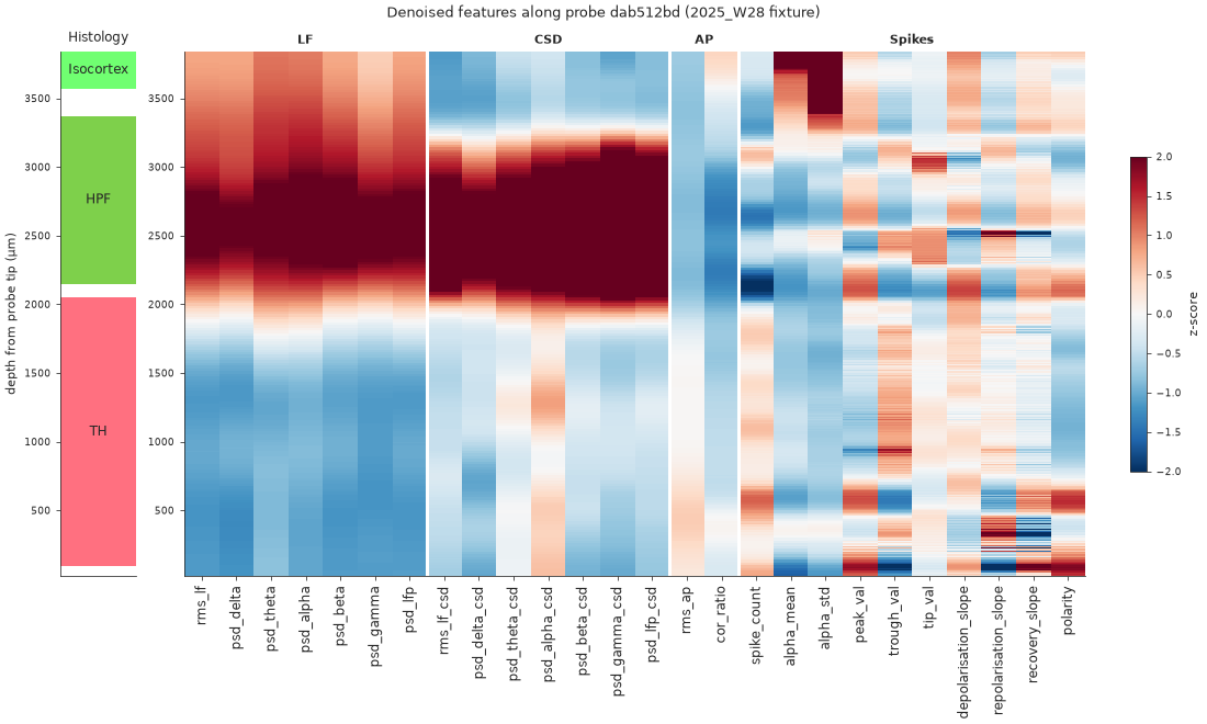
Features along the probe
Every feature of a probe against depth, beside the histology.
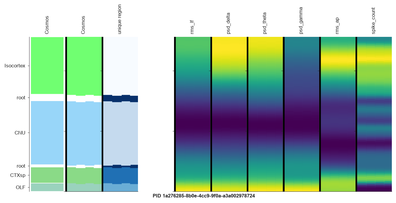
Feature strips on the probe geometry
A few features drawn on the channel layout, region colours alongside.
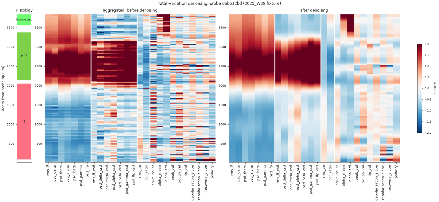
Before and after denoising
What the total-variation filter removes, and the boundaries it keeps.
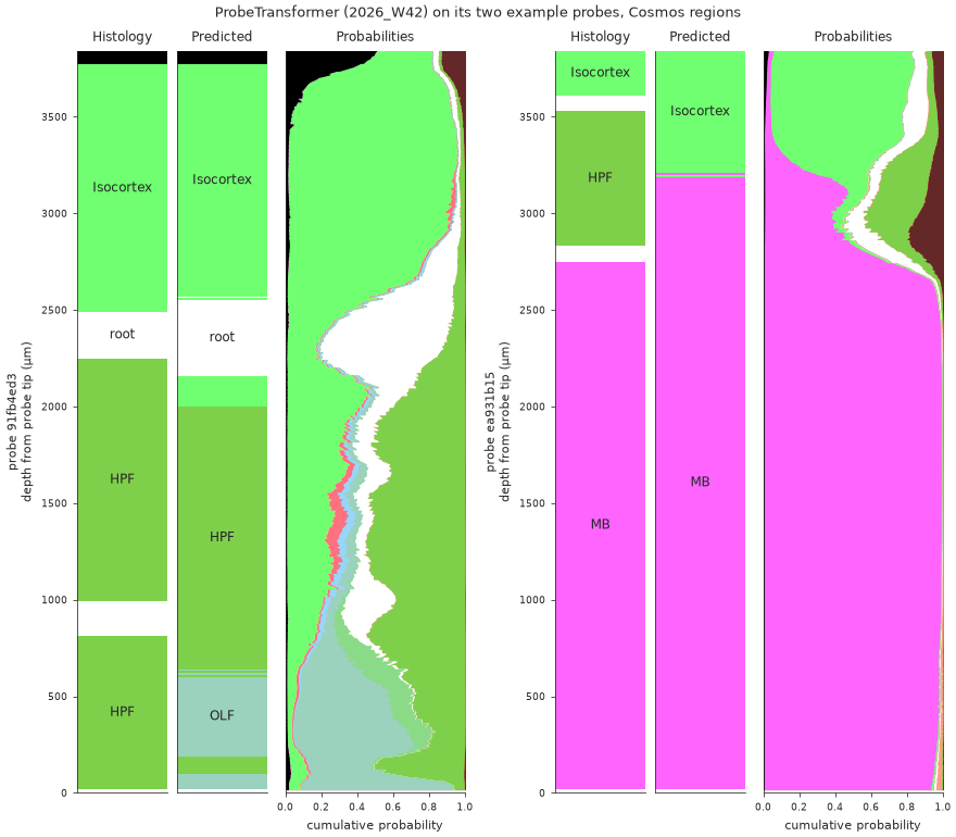
Region predictions along the probe
Histology, predicted region and the full posterior, against depth.
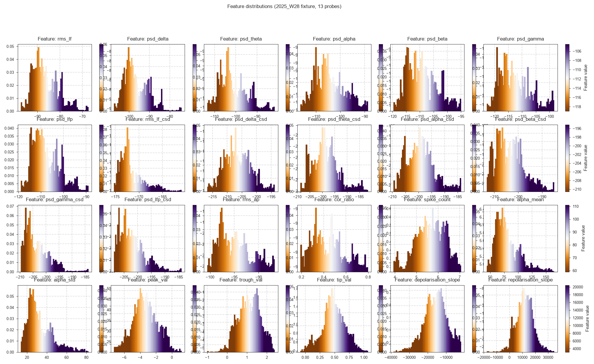
Feature distributions
The first check when a model behaves oddly on your data.
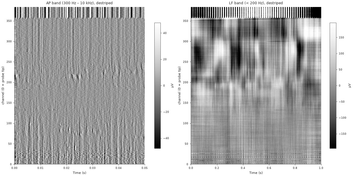
Raw and destriped voltage
The AP and LF snippets the features are computed on.
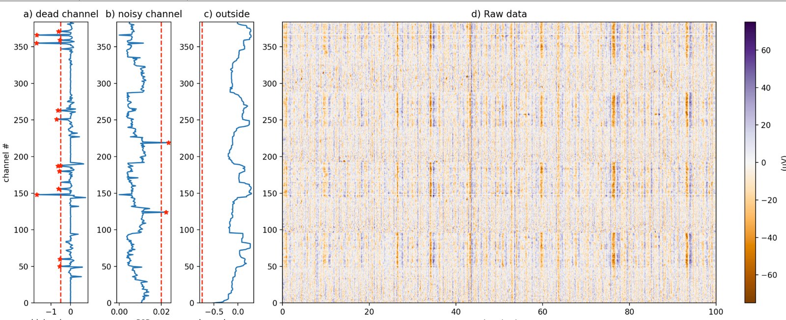
Bad channels
Why a channel is labelled dead, noisy or outside the brain.
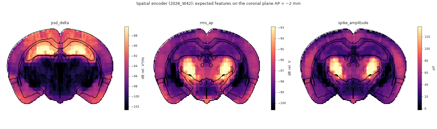
Atlas maps
What a channel at any position should record, on atlas slices.
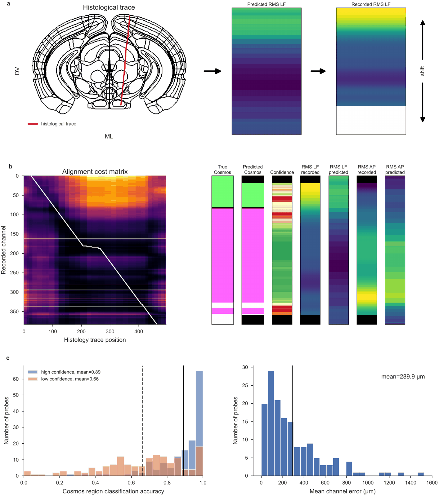
Alignment to histology
Recorded against predicted features along the histology track.
In the browser and in the GUI
Two IBL tools show the same data interactively:
- IBL Ephys Atlas viewer — the atlas, the predicted encoding volumes, gene expression atlases and the lipidome on linked brain slices, in the browser. It can also show a dataset of your own next to it.
- IBL alignment GUI — one probe at a time, features beside the histology, for aligning the probe. Its Channel Prediction plugin reads ibleatools features and adds the decoders’ predictions.