How to compute features from SpikeGLX AP/LF files
This guide computes electrophysiological features from a local Neuropixels recording saved by SpikeGLX — an AP-band and/or LF-band .bin or .cbin file with its .meta file.
This is the main entry point if you have your own Neuropixels data. For other formats see NWB and SpikeInterface Zarr; the workflow below is identical in all three cases — only the calculator changes.
Prerequisites
- ibleatools installed (see lite vs full)
- An AP and/or LF SpikeGLX file, each with its
.metafile alongside it
The lite install computes the lf, csd and ap families. The waveforms family needs DARTsort, which ships in the [full] extra:
pip install -e ".[full]"Compute features
The published models are trained on the per-channel median over several snippets spread through the recording, then denoised. compute_denoised_features builds that table from your files:
from ephysatlas.feature_calculators import SpikeGLXFileFeatureCalculator

calc = SpikeGLXFileFeatureCalculator(
    ap_file="/data/probe00/_spikeglx_ephysData_g0_t0.imec0.ap.cbin",
    lf_file="/data/probe00/_spikeglx_ephysData_g0_t0.imec0.lf.cbin",
    name="subject42_probe00",
)

df = calc.compute_denoised_features(n_snippets=5, duration_ap=5.0, duration_lf=5.0)
print(df.index.names)   # ['pid', 'channel']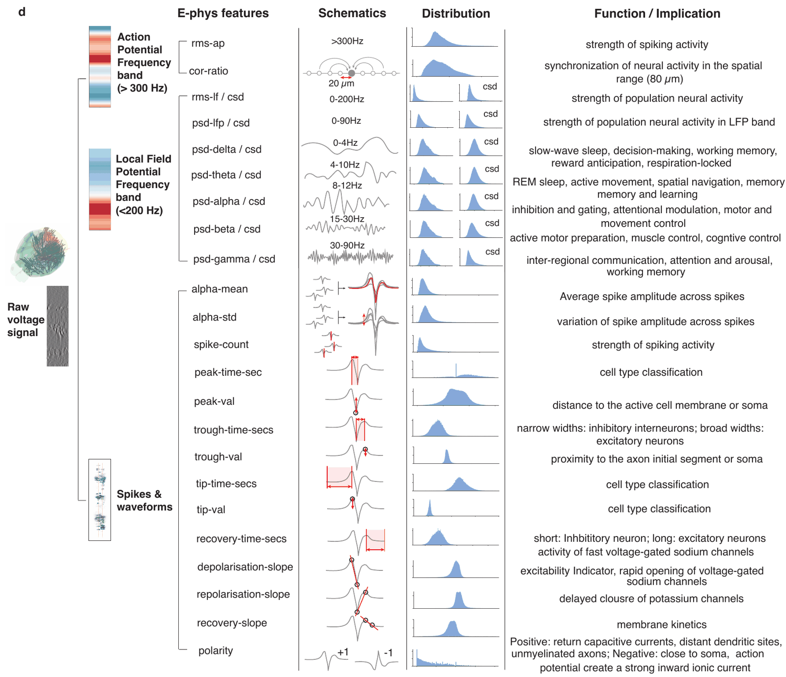
The snippets are spread over the recording, away from its first and last 5 minutes. The features come in four families: lf, csd, ap and waveforms (spike detection and waveform shape). Every family the files you passed support is computed, and the result is the same aggregated and denoised table as aggregate and denoise produces.
To compute only some families, pass options, for example to skip the spike features, which need the [full] install and take most of the time:
from ephysatlas.feature_calculators import FeatureComputationOptions

options = FeatureComputationOptions(features_to_compute=["lf", "csd", "ap"])
df = calc.compute_denoised_features(n_snippets=5, duration_ap=5.0, duration_lf=5.0,
                                    options=options)
The published region models need all four families, so keep the default if you plan to predict. Tune the computation lists the other options, such as output_dir to keep the snippet files. n_jobs= computes the snippets in parallel worker processes. Every calculator can be sent to a worker except IBLPIDFeatureCalculator, whose ONE client cannot, so it needs n_jobs=1.
Readers are opened lazily, so constructing the calculator touches no files until you ask for data.
The table records how it was made in df.attrs, and pandas keeps them in a parquet file:
df.attrs["snippet_windows"]   # [{'pid': ..., 't_start': ..., 'duration_ap': ..., 'duration_lf': ...}, ...]
df.attrs["features_version"]  # '2026_W42'
The ibleatools version and git commit of the code that computed the snippets are there too (ibleatools_distribution_version, and for an editable install ibleatools_git_commit_hash and ibleatools_git_is_dirty).
To compute a single snippet, choose the windows yourself, keep the snippet files, or work with a recording shorter than about 10 minutes, see tune the computation.
Only one band?
Pass just the file you have. Feature families that need the missing band are dropped automatically rather than erroring:
# LF only — 'lf' and 'csd' are computable, 'ap' and 'waveforms' are not
calc = SpikeGLXFileFeatureCalculator(lf_file="/data/probe00.lf.cbin")
df = calc.compute_denoised_features(n_snippets=5, duration_ap=0.0, duration_lf=5.0)
At least one of ap_file / lf_file is required; supplying neither raises ValueError.
Naming the recording
The recording name labels everything the calculator writes, and becomes the pid level of the (pid, channel) table. For a SpikeGLX calculator it defaults to the AP file stem (falling back to the LF stem, then "probe"). Override it when the stem is not a useful identifier — recommended, since SpikeGLX stems are often identical across probes:
calc = SpikeGLXFileFeatureCalculator(
    ap_file=..., lf_file=..., name="subject42_probe00"
)
From recording to brain regions
The whole path from two local files to a region per channel:
from ephysatlas import load_pretrained
from ephysatlas.feature_calculators import SpikeGLXFileFeatureCalculator

calc = SpikeGLXFileFeatureCalculator(
    ap_file="/data/probe00/_spikeglx_ephysData_g0_t0.imec0.ap.bin",
    lf_file="/data/probe00/_spikeglx_ephysData_g0_t0.imec0.lf.bin",
    name="subject42_probe00",
)
df = calc.compute_denoised_features(n_snippets=3, duration_ap=1.0, duration_lf=5.0)
df["outside"] = df["channel_labels"] == 3     # the one derived column the decoder needs

model = load_pretrained("int-brain-lab/ea-decoder-channel-xgboost", revision="2026_W42")
out = model.predict(df)
print(out["predicted_acronym"].value_counts())
A real run, on 30 seconds of AP and LF cut from IBL insertion 00a824c0-e060-495f-9ebc-79c82fef4c67 and saved as plain SpikeGLX files (384 channels, all four families, about three and a half minutes on a laptop CPU, most of it spike detection). Thirty seconds is shorter than the 5-minute margins of compute_denoised_features, so this run drew its three windows with the short-recording route instead:
from ephysatlas.feature_calculators import (
    SnippetWindow,
    compute_aggregated_features,
    get_snippet_start_times,
)

t_starts = get_snippet_start_times(30.0, n_snippets=3, snippet_duration=5.0,
                                   margin=0.0, method="linspace")   # [0, 12, 25]
df = compute_aggregated_features(calc, [SnippetWindow(t, 1.0, 5.0) for t in t_starts])
predicted_acronym
MB 161
Isocortex 79
root 58
TH 52
HPF 31
HY 3
mean prob 0.607 mean fold_agreement 0.823The published 2026_W42 aggregate of the same insertion, built from many more snippets, gives a cleaner picture with higher confidence — see predict regions. More snippets, and longer ones, make the estimates steadier.
Adding trajectory coordinates
Feature tables carry channel geometry (axial_um, lateral_um) out of the box. To also get anatomical target coordinates, pass the planned insertion trajectory:
traj_dict = {
    "x": -2243.1,      # µm, mediolateral
    "y": -1999.8,      # µm, anteroposterior
    "z": -361.0,       # µm, dorsoventral
    "depth": 4000.0,   # µm, insertion depth
    "theta": 15.0,     # degrees
    "phi": 180.0,      # degrees
}

from pathlib import Path

from ephysatlas.feature_calculators import FeatureComputationOptions

calc = SpikeGLXFileFeatureCalculator(
    ap_file=..., lf_file=..., traj_dict=traj_dict
)
options = FeatureComputationOptions(
    features_to_compute=["lf", "csd"],
    output_dir=Path("/data/features"),
    include_trajectory=True,
)
df = calc.compute_denoised_features(n_snippets=5, duration_ap=5.0, duration_lf=5.0,
                                    options=options)
This adds x_target / y_target / z_target to channels.pqt. Set require_trajectory=True to raise an error when the metadata is missing, instead of continuing without those columns.
Probe version
neuropixel_version (default 1) is forwarded to destriping, which applies version-specific spatial filtering. Set it to 2 for NP2 probes:
calc = SpikeGLXFileFeatureCalculator(ap_file=..., lf_file=..., neuropixel_version=2)Feature computation assumes one shank. A multi-shank recording (four-shank NP2, NP2.4) is not rejected: the csd family fails with a ZeroDivisionError in the Cadzow denoiser, and cor_ratio, the waveform features and the denoising mix the shanks without an error. See one shank per calculator for each step’s behaviour and the per-shank workaround for the LF families.
If your data is an IBL probe insertion
IBL recordings are addressed by probe insertion id (pid) and streamed through ONE, which needs an IBL account. IBLPIDFeatureCalculator is used in the same way, with the default n_jobs=1, since its ONE client cannot be sent to a worker process:
from one.api import ONE
from ephysatlas.feature_calculators import IBLPIDFeatureCalculator

one = ONE()
calc = IBLPIDFeatureCalculator(pid="00a824c0-e060-495f-9ebc-79c82fef4c67", one=one)
df = calc.compute_denoised_features(n_snippets=5, duration_ap=5.0, duration_lf=5.0)
Everything else on this page applies unchanged. The calculator also fills x_target / y_target / z_target from the best trajectory Alyx holds for the insertion: the micro-manipulator one, else the planned one, else the histology track (ephysatlas.feature_computation.PROVENANCE_PREFERENCE). An insertion with none of the three raises ValueError. If you only want the published IBL feature tables rather than to recompute them, download them instead — see load channel features.
Troubleshooting
ValueError: At least one of ap_file or lf_file must be provided — the constructor got neither file.
ValueError: Invalid feature sets requested — a name in features_to_compute is not one of lf, csd, ap, waveforms.
ValueError: No requested feature families match the available streams — you asked only for families that need a band you did not supply (e.g. ["ap"] with only an LF file).
A ModuleNotFoundError mentioning dartsort — waveforms features need the [full] extra.
A SEGFAULT during computation on macOS — a known PyTorch issue (pytorch#132372). Import torch first, before anything else in your script:
import torch # noqa: F401 — must precede the ephysatlas importsOr point the dynamic loader at your environment’s torch libraries:
export DYLD_LIBRARY_PATH=/path/to/venv/lib/python3.12/site-packages/torch/libOn Apple Silicon, torch and xgboost can also crash when both are loaded in one process. DARTsort brings torch, and the region decoder brings xgboost, so if the end-to-end example above crashes, compute the features in one process, save df with df.to_parquet(...), and predict in another.
AttributeError: 'function' object has no attribute '__wrapped__' from torch/_dynamo while computing waveforms (macOS) — on macOS the waveform step hides the MPS backend from DARTsort while it runs, and PyTorch 2.14 imported at that moment fails. Import torch._dynamo at the top of your script, before computing features:
import torch._dynamo # noqa: F401 — before computing waveform features on macOSNext steps
- Tune the computation — single snippets, snippet windows, per-feature parameters, bad-channel handling, and inspecting the destriped snippet
- Aggregate and denoise — what
compute_denoised_featuresdoes after computing the snippets - Predict brain regions — run the published decoder
- Plot features along the probe
- Which brain regions is my probe in? — this page as one step of the whole workflow
- The feature pipeline — what happens inside
compute_snippet