How to plot features along the probe
Electrophysiological features change systematically with depth — that structure is the whole reason a region decoder can work. This guide plots it three ways: each feature as a colour-coded strip down one probe beside the brain regions, every feature of a probe as one z-scored heatmap, and the distribution of every feature across a whole dataset.
Every figure on this page was produced by the code shown, run against the feature tables committed in this repository at tests/fixtures/features/2025_W28/ — 13 probes, 384 channels each. The script examples/plot_features_along_probe.py draws all of them.
Prerequisites
- A feature table indexed by
(pid, channel)— from your own recording or the published aggregates - The matching channel table, carrying
axial_um,lateral_umandatlas_id matplotlib
Prepare the data
The plotting functions want features and channel geometry in one DataFrame, plus a region-id column in the mapping you want to colour by. Merge on the (pid, channel) index, dropping the columns the two tables share so the merge produces no _x / _y suffixes:
from pathlib import Path

import pandas as pd
from iblatlas.regions import BrainRegions

path = Path("tests/fixtures/features/2025_W28")

df_features = pd.read_parquet(path / "raw_ephys_features_denoised.pqt")
df_channels = pd.read_parquet(path / "channels.pqt")

duplicate_cols = set(df_features.columns) & set(df_channels.columns)
df = df_features.merge(
    df_channels.drop(columns=duplicate_cols),
    how="inner",
    left_index=True,
    right_index=True,
)
print(df.shape)   # (4992, 42)

# Add a Cosmos-level region id, which the probe figure colours by.
# BrainRegions ships inside iblatlas — no download.
br = BrainRegions()
df["Cosmos_id"] = br.remap(
    df["atlas_id"].to_numpy(), source_map="Allen", target_map="Cosmos"
)BrainRegions, not ClassifierAtlas, for plotting
ephysatlas.data.read_features_from_disk does this merge and mapping for you, but it needs a brain_atlas and defaults to ClassifierAtlas(), which downloads the Allen template volumes — hundreds of megabytes you do not need to draw a figure. BrainRegions alone is enough to map and colour region ids, and it ships with iblatlas. The IBL documentation covers it in working with the atlas and the Allen, Beryl and Cosmos mappings in atlas mapping.
Features down one probe
figure_features_channel_space draws one panel per feature, each channel a rectangle at its true position on the probe, coloured by feature value — with the brain regions beside it for reference:
import ephysatlas.plots

pid = df.index.get_level_values("pid").unique()[0]
pid_df = df[df.index.get_level_values("pid") == pid].copy()

# Channel positions: lateral (x) then axial (y), in micrometres
xy = pid_df[["lateral_um", "axial_um"]].to_numpy()

features = ["rms_lf", "psd_delta", "psd_theta", "psd_gamma", "rms_ap", "spike_count"]

fig, axs = ephysatlas.plots.figure_features_channel_space(
    pid_df, features=features, xy=xy, pid=pid, br=br, mapping="Cosmos"
)
fig.savefig("features_along_probe.png", dpi=150, bbox_inches="tight")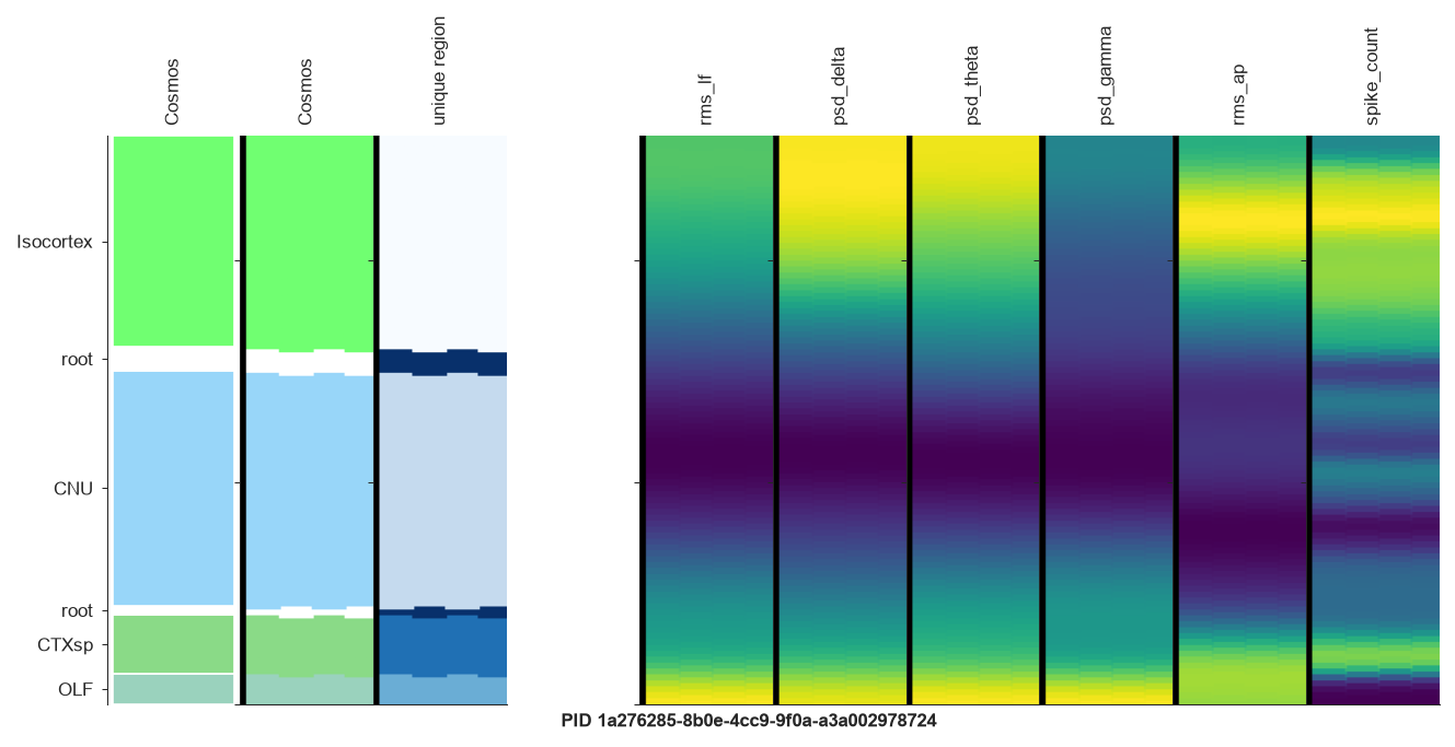
Read it left to right: the region labels and their Allen colours, the same regions as unique-colour bands, then one strip per feature. This probe passes through Isocortex, CNU, CTXsp and OLF, and rms_lf, psd_delta and rms_ap all shift visibly at those transitions.
xy must be ordered lateral-then-axial
xy is an [n_channels, 2] array whose first column is lateral_um and second is axial_um. Swap them and the figure renders without an error but places every channel at the wrong position.
Choosing what to show
features— any list of column names inpid_df. Panels appear in the order you give. Four to eight is comfortable; beyond that the panels get thin.mapping— the region map to colour by,"Cosmos"(coarse, 13 classes) or"Beryl"(finer). The function looks for a{mapping}_idcolumn, so remap first as shown above.br=None— omit the brain regions entirely. The three region panels are blanked and you get features only.cmap— any matplotlib colormap name. Defaults to"viridis".
Comparable colour scales
By default each panel scales its colours to its own min/max, so panels are not comparable to each other. Pin vmin / vmax to compare the same feature across probes:
fig, axs = ephysatlas.plots.figure_features_channel_space(
    pid_df, features=["rms_lf"], xy=xy, pid=pid, br=br, mapping="Cosmos",
    vmin=-95.0, vmax=-70.0,
)
Or pass a fitted scaler (anything with a .transform method, e.g. an sklearn StandardScaler) to z-score the features before display, which puts features with very different units on one visual footing:
from sklearn.preprocessing import StandardScaler

scaler = StandardScaler().fit(df[features])
fig, axs = ephysatlas.plots.figure_features_channel_space(
    pid_df, features=features, xy=xy, pid=pid, br=br, mapping="Cosmos",
    scaler=scaler,
)
Fit the scaler on the whole dataset, not one probe, or you have just removed the between-probe differences you wanted to see.
Looping over probes
from pathlib import Path

import matplotlib.pyplot as plt

outdir = Path("figures")
outdir.mkdir(exist_ok=True)

for pid in df.index.get_level_values("pid").unique():
    pid_df = df[df.index.get_level_values("pid") == pid].copy()
    fig, axs = ephysatlas.plots.figure_features_channel_space(
        pid_df,
        features=features,
        xy=pid_df[["lateral_um", "axial_um"]].to_numpy(),
        pid=pid,
        br=br,
        mapping="Cosmos",
    )
    fig.savefig(outdir / f"{pid}.png", dpi=150, bbox_inches="tight")
    plt.close(fig)   # or you will hold every figure in memory
All features as one heatmap
Strips get thin beyond eight features. To see every feature of a probe at once, figure_features_heatmap z-scores each feature over the whole dataset and draws the probe as an image, one row per channel sorted by depth and one column per feature, beside the histology:
feature_groups = {
    "LF": ["rms_lf", "psd_delta", "psd_theta", "psd_alpha", "psd_beta", "psd_gamma", "psd_lfp"],
    "CSD": ["rms_lf_csd", "psd_delta_csd", "psd_theta_csd", "psd_alpha_csd",
            "psd_beta_csd", "psd_gamma_csd", "psd_lfp_csd"],
    "AP": ["rms_ap", "cor_ratio"],
    "Spikes": ["spike_count", "alpha_mean", "alpha_std", "peak_val", "trough_val", "tip_val",
               "depolarisation_slope", "repolarisation_slope", "recovery_slope", "polarity"],
}

pid = "dab512bd-a02d-4c1f-8dbc-9155a163efc0"   # crosses Isocortex, HPF and TH

fig, axs = ephysatlas.plots.figure_features_heatmap(
    df_features, pid, channels=df_channels, feature_groups=feature_groups
)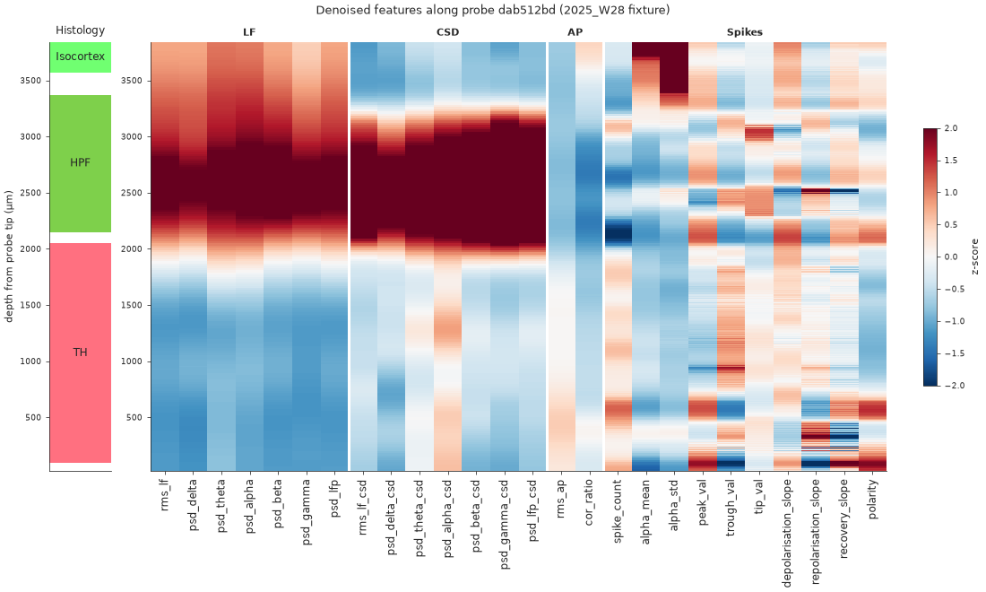
dab512bd as a z-scored heatmap: 26 features (columns), grouped by band, against depth, beside the histology. The LF and CSD bands light up in the hippocampus (HPF) and drop in the thalamus (TH), and the spike features change at the same boundaries.The histology bar takes the channel table’s Allen atlas_id and draws it at the Cosmos level (mapping). Leave out feature_groups to draw every feature the table has, grouped by family: LF, CSD, AP and spikes.
Two defaults matter. The mean and standard deviation of the z-score are taken over every probe of the table, for the same reason as the scaler above; pass mean and std to use other statistics. And the colour range is clipped at ±2 (vmin, vmax): the LF and CSD power of the hippocampus is several standard deviations above the rest of the brain and would otherwise wash out every other contrast.
Each part of the figure can be turned off with show_histology, show_colorbar, show_group_labels and show_feature_names. The axes come back by name (axs["histology"], axs["features"], axs["colorbar"]), to adjust them afterwards.
Before and after denoising
The same heatmap over the aggregated table (raw_ephys_features.pqt) and over the denoised one shows what the total-variation filter does: channel-to-channel noise goes, region boundaries stay sharp.
from ephysatlas.features import EphysTransformer

features = [f for group in feature_groups.values() for f in group]
df_raw = pd.read_parquet(path / "raw_ephys_features.pqt")

# Same units as the denoised table, so the two panels share one colour scale
transformer = EphysTransformer()
transformer.fit(df_raw[features])
df_raw_t = transformer.transform(df_raw[features])

# One panel per table, both z-scored with the statistics of the first
fig, axs = ephysatlas.plots.figure_features_heatmap(
    {"aggregated, before denoising": df_raw_t, "after denoising": df_features},
    pid,
    channels=df_channels,
    feature_groups=feature_groups,
    show_group_labels=False,
)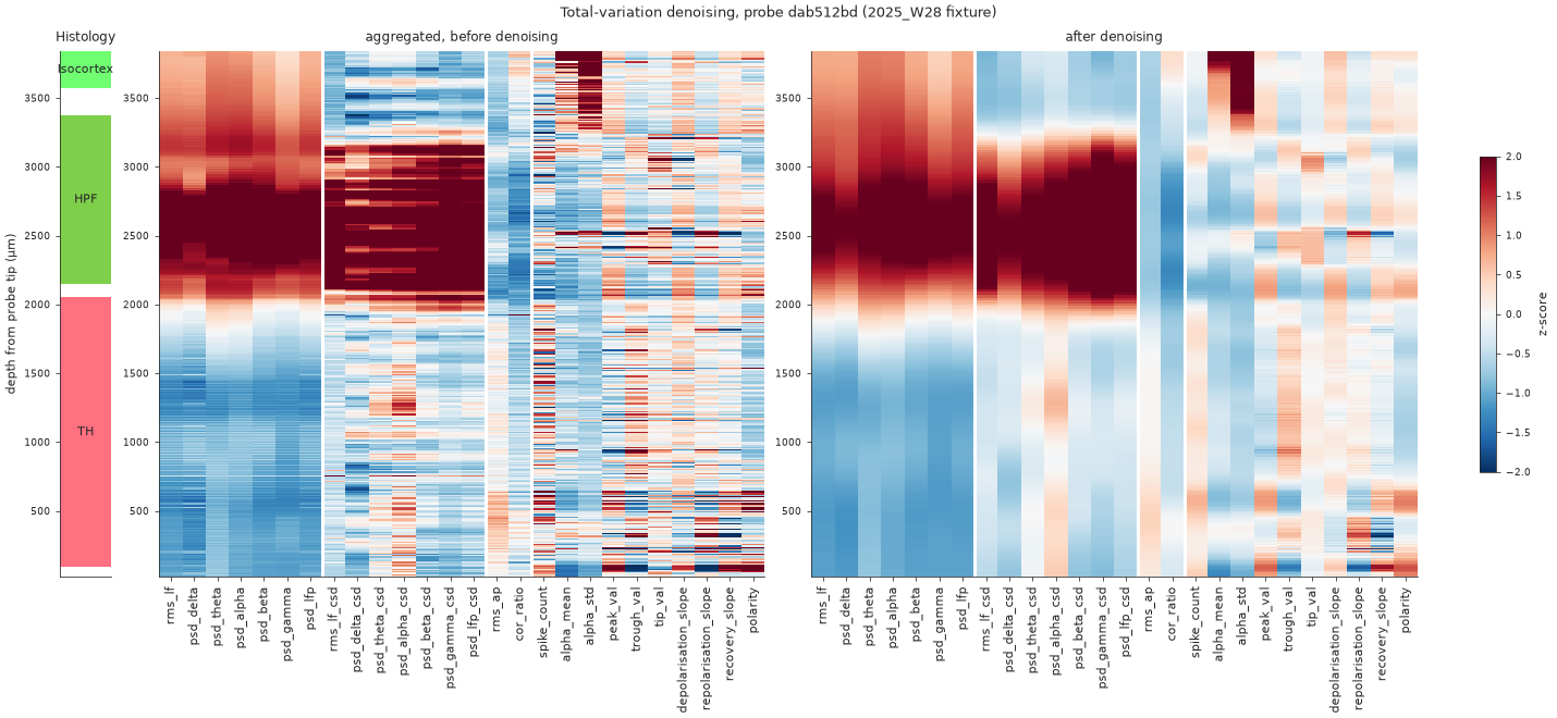
dab512bd, aggregated (left) and denoised (right), on one colour scale. The raw table was first put in the denoised units with ephysatlas.features.EphysTransformer (rms to dB, spike rate to log2), so the only difference left is the filter.See aggregate and denoise for the step itself.
Feature distributions across a dataset
plot_features_distributions gives the complementary view — the marginal distribution of each feature over every channel, with no depth information:
features_24 = [
    "rms_lf", "psd_delta", "psd_theta", "psd_alpha", "psd_beta", "psd_gamma",
    "psd_lfp", "rms_lf_csd", "psd_delta_csd", "psd_theta_csd", "psd_alpha_csd",
    "psd_beta_csd", "psd_gamma_csd", "psd_lfp_csd", "rms_ap", "cor_ratio",
    "spike_count", "alpha_mean", "alpha_std", "peak_val", "trough_val",
    "tip_val", "depolarisation_slope", "repolarisation_slope",
]

fig, axs = ephysatlas.plots.plot_features_distributions(
    df, x_list=features_24,
    title="Feature distributions (2025_W28 fixture, 13 probes)",
)
fig.savefig("features_distributions.png", dpi=150, bbox_inches="tight")
peak_val and trough_val exist in this 2025_W28 fixture, but not in the 2026_W42 denoised tables, which carry the spike-shape columns instead. On those tables, plot spike_amplitude and spike_width_secs in their place.
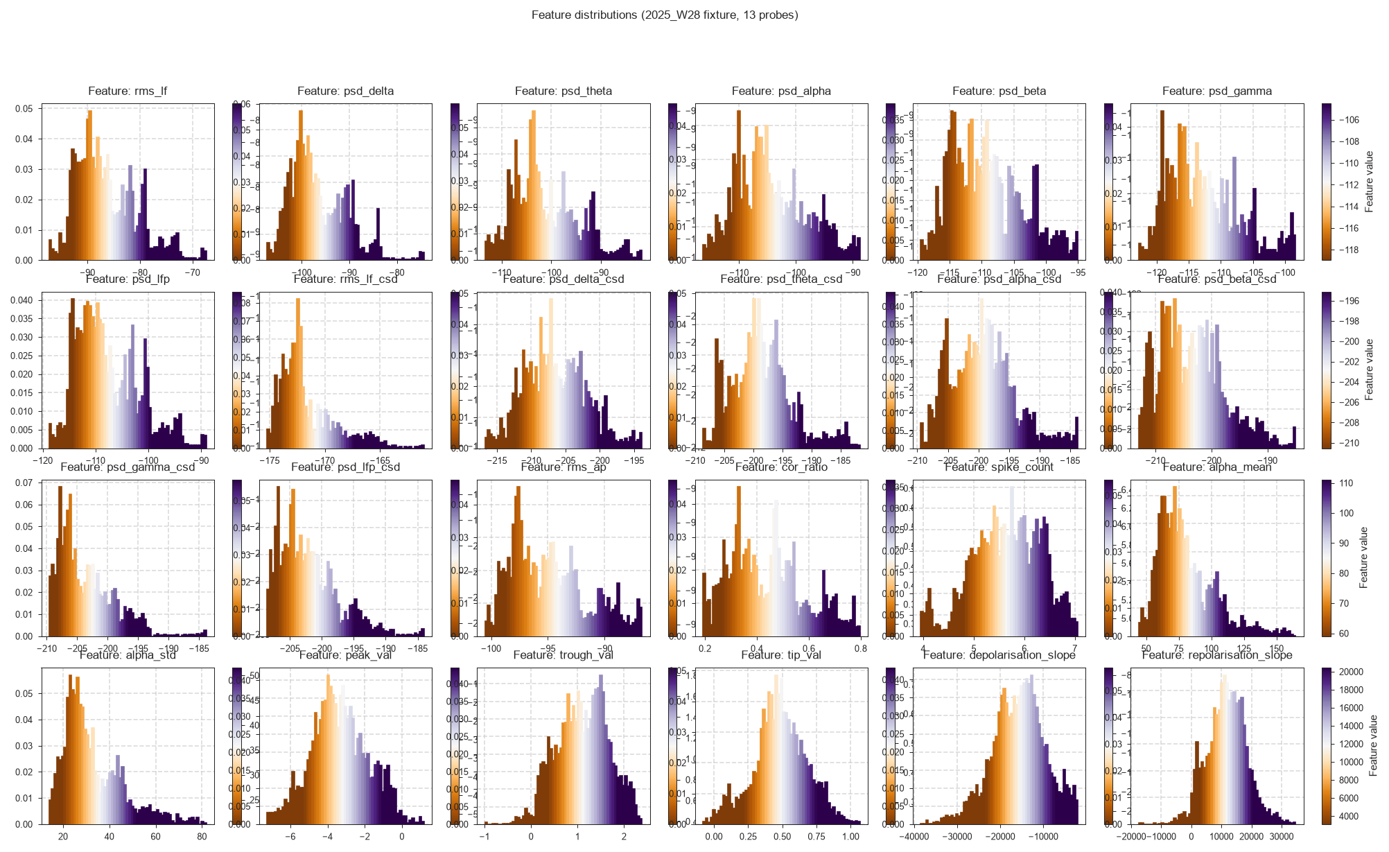
When a model gives unexpected results on your data, compare your distributions with these: a units problem or a badly scaled feature shows up as a shifted distribution.
The layout is a fixed 4×6 grid of histogram-plus-colorbar pairs, so it holds exactly 24 features. Fewer leaves blank panels; more than 24 raises IndexError — split the list across several calls instead. Features absent from the DataFrame are skipped with a warning rather than raising, and do not consume a panel.
Omit x_list entirely and it uses ephysatlas.features.voltage_features_set().
The values are in denoised units
Note the scales above: rms_lf sits near −90 and psd_* between −100 and −210, because raw_ephys_features_denoised.pqt stores rms_ap and rms_lf in dB and spike_count in log2. Plot raw_ephys_features.pqt instead and rms_lf comes out in volts, around 1e-5.
The two are not comparable, so a model trained on denoised features must be given denoised features. See aggregate and denoise.
Troubleshooting
KeyError: 'Cosmos_id' — figure_features_channel_space looks for a {mapping}_id column. Add it with br.remap(...) as shown, or pass br=None to skip the region panels.
The figure is drawn but channels are in the wrong places — xy columns are swapped. Lateral first, axial second.
A feature panel is uniformly one colour — that feature is constant or all-NaN for this probe. Check pid_df[feature].describe().
Warnings that a feature was not found and skipped — plot_features_distributions skips missing columns rather than raising. Check the names against df.columns.
Nothing renders in a script — matplotlib needs a backend. In a headless environment set matplotlib.use("Agg") before importing pyplot and save to file rather than calling plt.show().
Next steps
- Region predictions along the probe — put predictions beside these features
- Predict brain regions — run the decoders
- Feature list reference — what each feature measures
- Core concepts — why the denoised units differ
figure_features_channel_spaceAPI andfigure_features_heatmapAPI