How to predict brain regions
Two published decoders give each recording channel one of 13 Cosmos-level brain regions, from its electrophysiological features:
| decoder | Hugging Face repo | reads | agreement column |
|---|---|---|---|
| ProbeTransformer | int-brain-lab/ea-decoder-channel-transformer |
A whole probe at once, with depth along the probe | seed_agreement, over 5 seeds |
| XGBoost | int-brain-lab/ea-decoder-channel-xgboost |
Each channel on its own | fold_agreement, over 5 folds |
The ProbeTransformer attends across all channels of a probe, using depth along the probe (axial_um) as its positional signal, so a channel’s prediction can use the channels above and below it. The XGBoost decoder sees each channel independently.
This guide uses the ProbeTransformer. The XGBoost decoder takes the same table and returns the same columns; predict with XGBoost covers what differs.
If you have not loaded a model yet, start with how to download a published model.
What the decoders need
from ephysatlas import load_pretrained

transformer = load_pretrained(
    "int-brain-lab/ea-decoder-channel-transformer", revision="2026_W42"
)

print(transformer.inputs["index"])             # ['pid', 'channel']
print(len(transformer.inputs["features"]))     # 51
print(transformer.inputs["position_column"])   # axial_um
print(transformer.config["region_map"])        # Cosmos
Three requirements:
- A DataFrame indexed by
(pid, channel). - Every column in
transformer.inputs["features"], plus the position columnaxial_um.predictraisesKeyErrornaming any that are absent. - Features that are aggregated and denoised for this model’s vintage — see aggregate and denoise. Denoising returns
rms_apandrms_lfin dB andspike_count(a rate, in spikes/s) in log2, and the decoders expect those units.predictcannot check this: a raw single-snippet table has the right column names and the wrong units, so it runs without an error and returns wrong regions.
Prepare the table
The denoised table, raw_ephys_features_denoised.pqt, has every required column except outside, a boolean derived from channel_labels == 3 at read time rather than stored. Passing the denoised table straight to predict raises:
KeyError: "1 column(s) required by this model are missing from the input DataFrame:
['outside']. Expected the features plus the 'axial_um' position column."
This holds for the published ea_active/2026_W42 aggregate and for a table computed locally with compute_denoised_features.
There are three ways to get a complete table. For a downloaded vintage, the simplest is the pre-merged file, which already contains outside:
from pathlib import Path

import pandas as pd

path_features = Path("/data/features/ea_active/2026_W42/agg_full")   # from download_tables

df = pd.read_parquet(path_features / "df_all_cols_merged.pqt")
Or let read_features_from_disk derive it:
import ephysatlas.data, ephysatlas.anatomy

df = ephysatlas.data.read_features_from_disk(
    path_features, brain_atlas=ephysatlas.anatomy.ClassifierAtlas()
)
Or derive it yourself, with no atlas download:
df = pd.read_parquet(path_features / "raw_ephys_features_denoised.pqt")
df["outside"] = df["channel_labels"] == 3
Predict with the ProbeTransformer
out = transformer.predict(df)

print(out[["predicted_acronym", "prediction_probability", "seed_agreement"]].head())
out is indexed like df, one row per channel. Channels with any non-finite feature are dropped with a warning, so out can have fewer rows than df.
A real run on one probe of ea_active/2026_W42 (00a824c0-e060-495f-9ebc-79c82fef4c67, 384 channels, all returned):
predicted_acronym
MB            201
Isocortex     128
void           29
void_fluid     19
HPF             7

mean prob 0.816   mean seed_agreement 0.902
To try it with no data of your own, use the example the model ships, 768 channels from two probes:
sample = transformer.path_model / "example" / "features_sample.parquet"
out = transformer.predict(pd.read_parquet(sample))
Reading the output
| column | meaning |
|---|---|
predicted_acronym |
Winning region as an Allen acronym |
predicted_atlas_id |
The same region as a numeric Allen structure id |
prediction_probability |
Probability of the winning class, averaged over the seed models |
seed_agreement |
Fraction of seed models that voted for the winner |
p_<acronym> |
One column per class, averaged over the seed models |
The XGBoost decoder returns the same columns, averaged over its fold models, with fold_agreement in place of seed_agreement.
Both 2026_W42 decoders predict the same 13 Cosmos-level classes:
print(transformer.config["class_acronyms"])
# ['void', 'MB', 'Isocortex', 'CB', 'TH', 'CNU', 'OLF', 'CTXsp', 'root', 'HB',
#  'HPF', 'HY', 'void_fluid']
Note that void and void_fluid are real classes: the model can say a channel is outside brain tissue, which is useful for finding where a probe entered and exited.
Two different kinds of uncertainty
prediction_probability and seed_agreement answer different questions:
| probability | agreement | interpretation |
|---|---|---|
| high | high | Confident and consistent — trust it |
| low | high | Every seed agrees this channel is ambiguous, likely a region boundary |
| low | low | The seeds disagree; the model has no coherent answer here |
| high | low | Rare and suspicious — inspect the channel |
For the XGBoost decoder, read the folds for the seeds.
# Keep only channels the ensemble agrees on
confident = out[(out["prediction_probability"] > 0.5) & (out["seed_agreement"] >= 0.8)]
print(f"{len(confident)} / {len(out)} channels confidently assigned")
Filter on these two columns before using the predictions. On the probe above, 314 of the 384 channels pass this filter.
The full probability distribution
The p_<acronym> columns give the whole posterior, not just the winner:
prob_cols = [c for c in out.columns if c.startswith("p_")]
print(out[prob_cols].head())

# Runner-up per channel — often the anatomically adjacent region
top2 = out[prob_cols].apply(
    lambda r: r.nlargest(2).index[1].removeprefix("p_"), axis=1
)
Predict with XGBoost
The XGBoost decoder predicts each channel from its own features alone. It takes the same table:
xgb = load_pretrained(
    "int-brain-lab/ea-decoder-channel-xgboost", revision="2026_W42"
)

print(len(xgb.inputs["features"]))   # 48
print(xgb.config["accuracy"])        # 0.6124

out_xgb = xgb.predict(df)
print(out_xgb[["predicted_acronym", "prediction_probability", "fold_agreement"]].head())
What differs from the ProbeTransformer:
- Its 48 features include
channel_labelsbut not the four spike-shape columns (spike_width_secs,predepolarisation_width_secs,spike_amplitude,peak_to_trough_ratio_log), and it does not needaxial_um. - It returns every row:
out_xgbis indexed exactly likedf. - The release ships five cross-validation fold models plus one model trained on all channels, so the agreement column is
fold_agreement. - It can denoise raw aggregated features inside
predict(below).
On the same probe (352 of 384 channels pass the confidence filter above):
predicted_acronym
MB            197
Isocortex     138
void           28
HPF            13
void_fluid      8

mean prob 0.779   mean fold_agreement 0.930
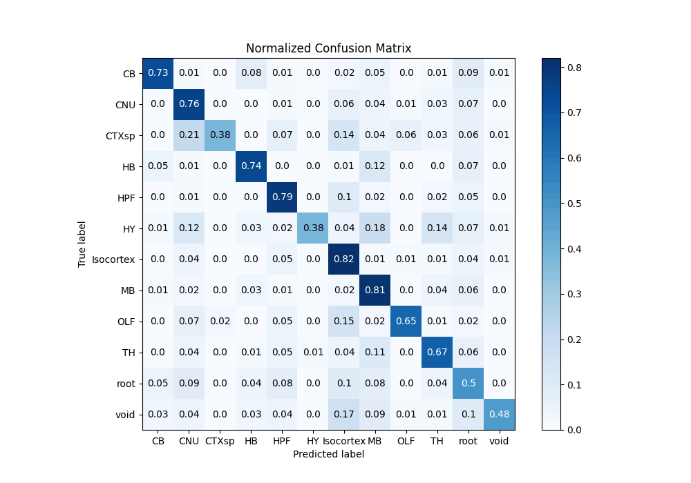
Its manifest records a held-out accuracy of 0.61 across the 13 classes. The accuracy is not the same for every region. The confusion matrix shows which regions are reliable and what the others are mistaken for:
Its shipped example holds 500 channels from 393 probes:
sample = xgb.path_model / "example" / "features_sample.parquet"
out_xgb = xgb.predict(pd.read_parquet(sample))
On macOS, run the two decoders in separate processes or with OMP_NUM_THREADS=1: see troubleshooting.
Denoising inside predict
If your table holds raw aggregated features, the XGBoost decoder can denoise them for you:
out_xgb = xgb.predict(df_raw, denoise=True)Leave denoise=False (the default) when your features are already denoised. Denoising twice degrades them. The ProbeTransformer has no such option.
Prefer denoising up front with produce_output_dataframes: you get the denoised table on disk for inspection, and you can reuse it across models.
Ensemble or global
Both decoders ship several models and average them by default. estimator= picks between the average and a single model:
out = transformer.predict(df, estimator="ensemble")   # default
out = transformer.predict(df, estimator="global")
"ensemble" (default) |
"global" |
|
|---|---|---|
| ProbeTransformer | Averages the 5 seed models | The first seed alone |
| XGBoost | Averages the 5 fold models | The single model trained on all channels |
| Cost | 5 forward passes | 1 forward pass |
| Agreement column | Real value in [0, 1] | NaN |
The agreement column is NaN for global: a single model has nothing to agree with, and 1.0 would suggest that all the models agreed when only one was used. For XGBoost, the ensemble is also slightly better calibrated.
The two estimators disagree on some channels: 9.6 % for the ProbeTransformer and 3.9 % for XGBoost on the probe above. Use the same estimator throughout an analysis.
Joining predictions onto your data
Prediction columns are namespaced so the join is always safe:
joined = df.join(out)Both the channel feature table and the cluster table already carry histology-derived acronym and atlas_id columns. Bare output names would collide on join and overwrite the histology columns on assignment without a warning. predicted_acronym / predicted_atlas_id cannot.
To compare the predictions with histology, you need a table that carries it: the pre-merged file or the output of read_features_from_disk, not the denoised table alone. Their acronym and atlas_id columns are Allen regions, while the decoders predict Cosmos regions, so compare against Cosmos_id:
labelled = df.join(out, how="inner")   # inner: out can have fewer rows than df
match = labelled["predicted_atlas_id"] == labelled["Cosmos_id"]
print(f"agreement with histology: {match.mean():.1%}")
Plotting the result
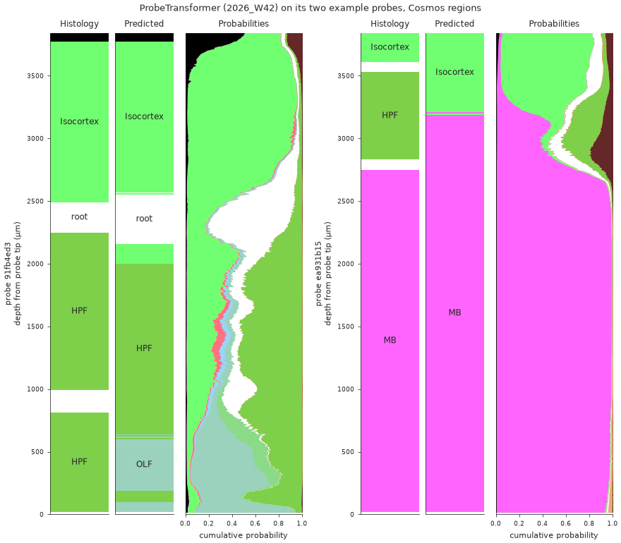
plot_cumulative_probas draws the full posterior as stacked bands down the probe, in Allen region colours:
import matplotlib.pyplot as plt
import numpy as np
import ephysatlas.plots
from ephysatlas.anatomy import NEW_VOID, ClassifierRegions

# The class list includes void_fluid (id 2000), unknown to plain BrainRegions
regions = ClassifierRegions()
regions.add_new_region(NEW_VOID)

# One probe at a time, sorted by depth. Join first: out can have fewer rows than df
pid = out.index.get_level_values("pid")[0]
probe = df[["axial_um"]].join(out, how="inner").xs(pid, level="pid").sort_values("axial_um")

# The p_<acronym> columns are in class order, so they align with config["classes"]
prob_cols = [f"p_{a}" for a in transformer.config["class_acronyms"]]

fig, ax = plt.subplots(figsize=(3, 8))
ephysatlas.plots.plot_cumulative_probas(
    probas=probe[prob_cols].to_numpy(),
    depths=probe["axial_um"].to_numpy(),
    aids=np.asarray(transformer.config["classes"]),   # one id per class, not per channel
    regions=regions,
    ax=ax,
    legend=True,
)
ax.set(xlabel="cumulative probability", ylabel="depth (µm)")
plt.show()
Three things to get right here: aids is one atlas id per class (13 of them), not one per channel; ax must be supplied — the function draws onto the axes you give it and returns it; and regions must know void_fluid, or its band is missing from the plot (the default is plain BrainRegions).
See plotting features along the probe for the depth-resolved feature view beside the predictions, and region predictions along the probe for the comparison with histology.
Troubleshooting
KeyError listing feature columns — your table is missing those columns. Usually a feature family you did not compute; the 2026_W42 decoders need all four (lf, csd, ap, waveforms), and waveforms needs the [full] extra. A list of peak_val, trough_val, peak_time_secs and friends means the opposite mismatch: an older model on a table from ephysatlas 0.9.0 or later, which no longer has those columns. Use the 2026_W42 model. A list of *_bpr columns means a table computed before ephysatlas 0.10.0, whose first-difference columns are *_csd_diff1; recompute the features.
ValueError about the feature-order digest — the manifest’s feature list no longer matches its recorded hash, meaning the model directory has been edited. Re-download it.
Predictions look uniformly wrong — check three things in order: model.selftest() passes; your features are denoised; the feature vintage matches model.index["vintage"].
Everything predicted void or root — often a sign the input is raw rather than denoised, so the feature values sit far outside the training distribution.
transformer.predict never returns after the XGBoost decoder ran in the same process (macOS) — XGBoost and PyTorch each load their own OpenMP runtime, and the second one deadlocks. Importing torch first instead crashes the XGBoost predict. Start Python with OMP_NUM_THREADS=1 (OMP_NUM_THREADS=1 python my_script.py), or run the two decoders in separate processes. Seen with XGBoost 3.4.1 and PyTorch 2.14 on Apple Silicon.
Next steps
- Which brain regions is my probe in? — the whole workflow, including alignment to histology
- Plot features along the probe
- Region predictions along the probe
- Predict features from position — the inverse model
- Model manifest reference
ProbeTransformerClassifierAPI andRegionClassifierAPI