How to tune feature computation

Everything on this page applies to every calculator — SpikeGLX, NWB, Zarr, IBL PID, and the LF-only LFPack and NumPy sources alike. The source-specific pages cover the usual call, compute_denoised_features; this one covers controlling it: computing a single snippet, choosing the snippet windows, and changing how each snippet is computed. The same options go to compute_snippet and to compute_denoised_features, which applies them to every snippet.

Compute a single snippet

compute_denoised_features is built on a smaller call, calc.compute_snippet(window, options), which computes the features of one snippet from three objects:

A calculator — where the data comes from: any of the calculators above.
A SnippetWindow — which slice of time to compute over.
A FeatureComputationOptions — which feature families, where to write, and any per-feature parameters.

from pathlib import Path

from ephysatlas.feature_calculators import FeatureComputationOptions, SnippetWindow

window = SnippetWindow(t_start=300.0, duration_ap=1.0, duration_lf=1.0)

options = FeatureComputationOptions(
    features_to_compute=["lf", "csd"],
    output_dir=Path("/data/features"),
)

result = calc.compute_snippet(window, options)   # calc: any calculator

print(result.features.shape)
print(result.computed_features)   # ('lf', 'csd')

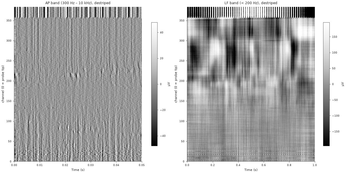
To see the voltage this window covers, destriped as the features see it, calc.get_destriped_snippet(window) returns it without computing any feature; see inspecting the destriped data.

The snippet window

SnippetWindow sets one start time and independent durations per band:

field	default	meaning
`t_start`	`0.0`	Start time in seconds from the beginning of the recording
`duration_ap`	`5.0`	Length of the AP-band snippet, in seconds
`duration_lf`	`25.0`	Length of the LF-band snippet, in seconds

The bands get different durations because they are informative on different timescales: LF features want a long window to resolve low-frequency power, while AP/waveform features are expensive and converge quickly. Setting a duration to 0.0 skips that band.

Start well after t_start=0 — the first seconds of a recording often contain settling artefacts. 300.0 is a common choice.

Start small

Features on a 1-second snippet of one probe take seconds; waveform features on a long window take minutes to hours. Get the call working with duration_ap=1.0, duration_lf=1.0 and features_to_compute=["lf"] before scaling up.

Feature families

features_to_compute accepts any subset of four families:

family	band	what it produces
`"lf"`	LF	Band power, RMS, spectral-decay parameters
`"csd"`	LF	The same measures on the current-source density
`"ap"`	AP	AP-band RMS and channel cross-correlation
`"waveforms"`	AP	Spike detection and waveform shape (needs `[full]`)

Leave features_to_compute=None to compute every family the available bands support. An unknown name raises ValueError listing the valid options.

See the feature list reference for the exact columns each family emits.

What you get back

compute_snippet returns a FeatureComputationResult:

result.features            # pd.DataFrame — one row per channel, with a `channel` column
result.computed_features   # families actually recalculated in this call
result.cached_features     # families loaded from existing files on disk
result.probe_level_dir     # .../features/<name>/
result.snippet_level_dir   # .../features/<name>/probe_<name>_<t_start>_<dur_ap>_<dur_lf>/
result.provenance          # versions + parameters stamped onto the written files
result.manifest_record     # one row for the aggregation step

<name> is the calculator’s recording name, the pid of the aggregated table; each calculator page gives its default.

On-disk layout

With output_dir set, files are written in a two-level structure:

/data/features/
└── subject42_probe00/                                      ← probe level (the `name`)
    ├── channels.pqt                                        channel metadata + geometry
    └── probe_subject42_probe00_000300.0_01.0_01.0/         ← snippet level
        ├── lf_features.pqt
        └── csd_features.pqt

The snippet directory name encodes t_start, duration_ap and duration_lf, so different windows over the same recording sit side by side and never overwrite each other. Each *_features.pqt carries the run’s provenance in its .attrs.

Leave output_dir=None and nothing is written — result.features is returned in memory and probe_level_dir / snippet_level_dir come back as None.

Choose the snippet windows

compute_denoised_features draws the snippet start times for you. To choose them yourself, draw the start times, then aggregate:

from ephysatlas.feature_calculators import (
    SnippetWindow,
    compute_aggregated_features,
    get_snippet_start_times,
)

# seconds; a missing band has no duration
duration_s = min(d for d in calc.available_duration() if d is not None)
t_starts = get_snippet_start_times(
    duration_s, n_snippets=5, snippet_duration=5.0, margin=300.0
)
windows = [SnippetWindow(t, 5.0, 5.0) for t in t_starts]
df = compute_aggregated_features(calc, windows)

margin keeps the snippets away from both ends of the recording. method="stratified" (the default) draws one random start in each of n_snippets equal bins, reproducibly (seed=0); method="linspace" spaces them evenly.

Short recordings

compute_denoised_features keeps the default 5-minute margins, so a recording shorter than 10 minutes plus one snippet raises ValueError: Recording of ... s is too short for 300.0 s margins and 5.0 s snippets.

Overlapping snippets raise ValueError: Snippets starting at ... overlap (or log a warning with on_overlap="warn"). The stratified draw can place two starts closer than one snippet when the usable range is short: with margin=0, three 5-second snippets fail on a 20- or 25-second recording and fit on 30 seconds. On a short recording, draw the times with margin=0 and method="linspace", and call compute_aggregated_features:

t_starts = get_snippet_start_times(
    duration_s, n_snippets=3, snippet_duration=5.0, margin=0.0, method="linspace"
)

Write the snippets yourself

To keep every snippet on disk, and resume an interrupted run, loop over start times reusing the calculator:

output_dir = Path("/data/features")
options = FeatureComputationOptions(
    features_to_compute=["lf", "csd"],
    output_dir=output_dir,
    skip_saved_computation=True,   # resume instead of recomputing
)

results = []
for t_start in [300.0, 900.0, 1500.0, 2100.0]:
    window = SnippetWindow(t_start=t_start, duration_ap=1.0, duration_lf=1.0)
    result = calc.compute_snippet(window, options)
    print(t_start, result.computed_features, result.cached_features)
    results.append(result)

skip_saved_computation=True reuses feature files already present in the snippet directory, so an interrupted run resumes where it stopped instead of starting over.

Then combine the snippets into one per-channel table, the one the models actually consume. aggregate_snippets is the aggregation half of compute_aggregated_features; it reads the snippet files back, so the snippets need an output_dir:

from ephysatlas.feature_calculators import aggregate_snippets

df = aggregate_snippets(results)   # per-channel median, denoised, indexed by (pid, channel)

Aggregate and denoise explains each step, and how to aggregate snippets already on disk without the calculator.

Computation options

FeatureComputationOptions controls one compute_snippet call. Every field has a working default, so set only what you need to change.

What to compute, and where it goes

field	default	effect
`features_to_compute`	`None`	Families to compute: any of `"lf"`, `"csd"`, `"ap"`, `"waveforms"`. `None` computes everything the available bands support
`output_dir`	`None`	Root for the probe/snippet output tree. `None` writes nothing and returns features in memory only
`scratch_dir`	`None`	Scratch space for waveform extraction. `None` uses `dartsort/` in the system temp directory (`$TMPDIR`). Point this at a fast local disk when computing `waveforms`; a directory that cannot be created raises `OSError`

Caching and reruns

field	default	effect
`skip_saved_computation`	`False`	Reuse feature files already in the snippet directory instead of recomputing them
`recompute_channels`	`False`	Rewrite `channels.pqt` even when it exists
`save_waveforms`	`False`	Persist the waveform arrays, not just the derived features

skip_saved_computation=True is what makes a long multi-snippet run resumable. Which families were reused is reported back:

result = calc.compute_snippet(window, options)
print(result.computed_features)   # recalculated in this call
print(result.cached_features)     # loaded from disk

Trajectory metadata

field	default	effect
`include_trajectory`	`True`	Try to add `x_target` / `y_target` / `z_target` to the channel table
`require_trajectory`	`False`	Raise instead of continuing when that metadata is missing

Only the IBL PID calculator, and a SpikeGLX calculator given a traj_dict, have a trajectory to add. For every other source, leaving include_trajectory on only logs that no trajectory is available. If your pipeline depends on those coordinates, set require_trajectory=True so a missing trajectory raises an error instead of producing a table without those columns.

Destriping and bad channels

field	default	effect
`lf_k_filter`	`False`	Spatial-filter mode for LF destriping. `None` disables LF spatial filtering entirely
`skip_lf_destripe`	`False`	Skip LF destriping altogether, for LF that is already preprocessed and decimated (lfpack archives, arrays). Channel labels then come from the source’s channel table
`channel_labels`	`None`	Explicit per-channel bad-channel labels, overriding automatic detection
`extra_kwargs`	`{}`	Passed straight through to the underlying engine

By default the calculator resolves channel labels automatically — from stored labels, from the .cbin metadata, or by detecting them on the snippet. Pass channel_labels to override that. To disable bad-channel handling completely, pass an all-zero array:

import numpy as np

options = FeatureComputationOptions(
    features_to_compute=["lf"],
    channel_labels=np.zeros(384),   # every channel treated as good
)

That is useful when comparing against an external pipeline that does no bad-channel rejection, or when debugging a suspicion that detection is discarding good channels.

Per-feature parameters

feature_params reaches inside individual feature families. It accepts either the typed objects or an equivalent nested dict — these two are the same:

from ephysatlas.feature_calculators import CsdParams, FeatureParams

FeatureParams(csd=CsdParams(scale=False))
{"csd": {"scale": False}}

Only what you set changes; every other parameter keeps its default, and the default FeatureParams() reproduces the standard output exactly.

Tip

A misspelled name raises an error: an unknown family name raises ValueError and an unknown sub-parameter raises TypeError. The typed objects also let your editor catch it before you run the code.

LF parameters — `LfParams`

field	default	meaning
`bands`	`None`	Frequency bands for the LF spectral step. `None` uses the standard delta/theta/alpha/beta/gamma set
`decay_features`	`True`	Compute the PSD-decay (spectral parameterisation) features. The `csd` family never computes them on its CSD and BPR traces
`compute_rms_no_car`	`False`	Also emit `rms_lf_no_car` — LF RMS destriped without common-average referencing

from ephysatlas.feature_calculators import LfParams

options = FeatureComputationOptions(
    features_to_compute=["lf"],
    feature_params=FeatureParams(lf=LfParams(compute_rms_no_car=True)),
)

rms_lf_no_car is opt-in because CAR removes shared signal across channels; the no-CAR RMS retains it, which is informative for some analyses and misleading for others.

CSD parameters — `CsdParams`

field	default	meaning
`bands`	`None`	Frequency bands for the CSD spectral step
`decimate`	`10`	Temporal decimation applied before computing the CSD. `1` skips it
`scale`	`True`	Scale the spatial differences by the tissue conductivity and the intercontact distance (A/m³ for CSD, A/m² for BPR). `False` keeps the raw differences in V
`denoise`	`True`	Apply the Cadzow denoiser to the decimated LF before the CSD and BPR finite differences. Turn it off for LF that is already Cadzow-denoised, so it is not denoised twice
`cadzow_kwargs`	`None`	Overrides of the Cadzow parameters. `None` uses `features.cadzow_lfp_kwargs(geometry)`; `fs` and `h` cannot be overridden

LF-only sources whose LF is already decimated and denoised need CsdParams(decimate=1, denoise=False); see computing features from the archives.

options = FeatureComputationOptions(
    features_to_compute=["csd"],
    feature_params={"csd": {"scale": False}},
)

The Cadzow defaults depend on the probe layout. cadzow_lfp_kwargs returns the ibl-neuropixel LFP defaults: Gavish-Donoho shrinkage (shrinkage=2.25) on the full lateral × depth grid (fill_grid=True) for the NP1 checkerboard, and shrinkage=1.22 without grid filling for NP2, whose contacts already fill their grid. To see what a geometry gets, or to use the adaptive rank cut instead of the shrinkage:

import neuropixel
from ephysatlas.features import cadzow_lfp_kwargs

print(cadzow_lfp_kwargs(neuropixel.trace_header(version=1)))
# {'fill_grid': True, 'rank': 5, 'niter': 1, 'fmax': None, 'nswx': 64, 'ovx': 32,
#  'ppca_k': 2.0, 'shrinkage': 2.25}

rank_cut = CsdParams(
    cadzow_kwargs={"fill_grid": False, "shrinkage": None, "gap_threshold": 2.0, "fmax": 125}
)

Changing the Cadzow parameters changes every *_csd and *_bpr value, so the output no longer matches the published models.

Waveform parameters — `WaveformParams`

These are DARTsort detection parameters, and they need the [full] extra.

field	default	meaning
`n_jobs`	`0`	`0` runs in the main process (CUDA initialised in-process; GPU memory is not freed between calls). `1` runs in a worker subprocess, which frees GPU memory on exit but needs a working multiprocessing environment
`detection_threshold`	`4.0`	Peak detection threshold, in units of channel RMS
`spatial_dedup_radius_um`	`150.0`	Radius within which only the largest simultaneous peak is kept
`positive_temporal_dedup_radius_samples`	`7`	Samples around a trough in which positive peaks are suppressed
`residnorm_decrease_threshold`	`3.162`	Minimum residual-norm decrease for a detected spike to be subtracted

from ephysatlas.feature_calculators import WaveformParams

options = FeatureComputationOptions(
    features_to_compute=["waveforms"],
    scratch_dir="/fast/scratch",
    feature_params=FeatureParams(
        waveforms=WaveformParams(detection_threshold=5.0, n_jobs=1)
    ),
)

Warning

Changing detection_threshold changes spike_count and every waveform-shape feature — which means the result no longer matches what the published models were trained on. Keep the defaults if you intend to run a published model over the output.

Inspecting the destriped data

get_destriped_snippet runs the same destriping as compute_snippet but stops there, so you can look at the intermediate voltage without paying for feature computation:

snippet = calc.get_destriped_snippet(window)

snippet.raw.raw_ap      # (channels, samples) raw AP, volts — or None
snippet.raw.raw_lf      # (channels, samples) raw LF, volts — or None
snippet.raw.fs_ap       # AP sampling rate, Hz
snippet.raw.fs_lf       # LF sampling rate, Hz
snippet.des_ap          # destriped AP — or None
snippet.des_lf          # destriped LF — or None
snippet.geometry        # channel geometry used by the destriper
snippet.channel_labels  # bad-channel labels the destriper applied

If the features look wrong, plot raw against destriped to see whether destriping is the cause:

import matplotlib.pyplot as plt

fig, (ax_raw, ax_des) = plt.subplots(1, 2, figsize=(12, 6), sharey=True)
ax_raw.imshow(snippet.raw.raw_lf, aspect="auto", cmap="RdBu_r")
ax_raw.set(title="raw LF", ylabel="channel")
ax_des.imshow(snippet.des_lf, aspect="auto", cmap="RdBu_r")
ax_des.set(title="destriped LF")
plt.show()

get_destriped_snippet also accepts a DestripeOptions to vary lf_k_filter, ap_k_filter, neuropixel_version and nshank for the inspection alone, without touching your production options.

A destriped snippet drawn in grey, scaled on the typical channel: AP (first 50 ms) and LF. Raw and destriped voltage has the code, the destriping steps and the bad-channel figure.

Provenance

Every feature file written carries the run’s provenance in its pandas .attrs — package versions and the parameters used:

print(result.provenance)

import pandas as pd
df = pd.read_parquet(result.snippet_level_dir / "lf_features.pqt")
print(df.attrs)

This is how you establish, months later, which parameters produced a table on disk. When skip_saved_computation reuses a cached family, its file keeps the provenance of the run that originally created it — so a mixed directory records the provenance of each part separately.

Next steps

Aggregate and denoise — combine snippets into a model-ready table
Feature list reference — the columns each family emits
The feature pipeline — why destriping and denoising are separate steps
FeatureComputationOptions API

Compute a single snippet

The snippet window

Feature families

What you get back

On-disk layout

Choose the snippet windows

Write the snippets yourself

Computation options

What to compute, and where it goes

Caching and reruns

Trajectory metadata

Destriping and bad channels

Per-feature parameters

LF parameters — LfParams

CSD parameters — CsdParams

Waveform parameters — WaveformParams

Inspecting the destriped data

Provenance

Next steps

LF parameters — `LfParams`

CSD parameters — `CsdParams`

Waveform parameters — `WaveformParams`