Model families

Four model families, one load path. This page explains what each family does, why they are published differently, and how a single load_pretrained call serves all of them.

The four families

family	granularity	input	output	on the Hub
Region decoder	channel	Features	Brain region	`ea-decoder-channel-xgboost`
Whole-probe region decoder	channel	A probe’s features, with depth	Brain region per channel	`ea-decoder-channel-transformer`
Spatial encoder	channel	Position (`x`,`y`,`z`)	Features	`ea-encoder-channel`
Unit encoder	unit	Position (`x`,`y`,`z`); or a unit’s waveform, ACG and population coupling	Expected unit phenotype; or the unit’s latent and cell type	`ea-encoder-unit`

Region decoder — features in, region out

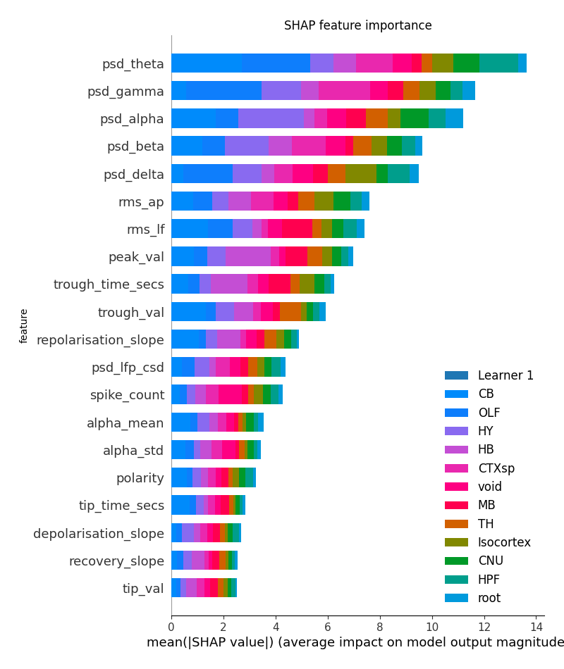
An XGBoost classifier over channel features, predicting one of 13 Cosmos-level brain regions per channel. Five cross-validation folds plus one all-data model ship together, so the agreement between folds (fold_agreement) is reported alongside the probability.

It answers “where is this channel?” from the recording alone. Its held-out accuracy is around 0.59 across 13 classes, well above chance but far from certain, so check fold_agreement before relying on a prediction.

Which features the region decoder relies on: mean absolute SHAP value per feature, split by the region it pushes towards. The LF band powers lead, then AP-band RMS and the waveform features.

Whole-probe region decoder — a probe in, regions out

The same question, answered for a whole probe at once. ProbeTransformerClassifier is a transformer with rotary position encoding that attends across all channels of a probe, using depth along the probe (axial_um) as its positional signal. A channel’s prediction can therefore use what the channels above and below it look like, which the per-channel decoder cannot.

A release ships one model per random seed — five for 2026_W42 — so its disagreement signal is seed_agreement rather than fold_agreement. Channels with any non-finite feature are dropped with a warning, so its output can be a subset of the input. See predict regions.

Spatial encoder — position in, features out

A transformer that predicts a channel’s features from where it sits in the brain. Two inputs: the anatomical context at those coordinates (MERFISH and AGEA gene/cell-expression PCA volumes) and the recorded features of nearby channels on other probes.

The encoder’s two inputs: the sparse recordings, and the MERFISH and AGEA molecular context everywhere. Together they give a dense map of each feature.

It runs in the opposite direction to the decoder: it predicts what a channel at a given position should record, so a large residual against the measured features is evidence that a probe is not where the trajectory places it. Drawn on an atlas slice, its predictions are a map of the brain’s electrophysiology: see atlas maps.

Neighbours come from other probes only (allow_same_probe: false), so a prediction for a probe already in the training bank does not use that probe’s own features. The current release also takes no coordinate input of its own (use_positions: false): position reaches the model only through the context sampled there and the neighbours found there. Queries are mirrored to the left hemisphere, as in training.

Unit encoder — position in, unit phenotype out

The unit-level model describes the spike-sorted units found at a brain location:

A multimodal autoencoder (UnitAutoencoder) embeds a unit’s multi-channel waveform, 3D autocorrelogram and population coupling (stPC) — 20 dimensions each — into a joint 60-dimensional latent: the unit’s phenotype.
A hierarchical Gaussian mixture over those latents. Thirty putative cell types, each split into at most ten sub-types of at least 20 training units — 300 sub-types in 2026_W42. Assignment is top-down, so a unit’s sub-type always lies inside its type.
At a position, the sub-type weights come from two networks of the molecular context there (MERFISH + AGEA PCA): one for the types, one for the sub-types’ shares within each type.
Each sub-type is read out through its training members: their mean waveform features, or one of them for a draw.

So, like the spatial encoder, its predict takes positions and returns the phenotype expected there. mixture_weights gives the cell-type composition and sample draws real training units. For your own units, encode, posterior and assign place them in the mixture. See predict unit phenotypes.

2026_W42 is the release of this model. The repository’s earlier tags hold a previous, flat-mixture model that this version of ephysatlas does not load.

One load path

Every family loads the same way:

from ephysatlas import load_pretrained

model = load_pretrained(repo_id, revision="2026_W42")
out = model.predict(df)

load_pretrained resolves the id to a directory, reads ephysatlas_model.json, and looks up model_class in a 1:1 table of wrapper builders:

`model_class`	wrapper
`xgboost.sklearn.XGBClassifier`	`RegionClassifier`
`ProbeTransformer`	`ProbeTransformerClassifier`
`NeighborInpaintingModel`	`SpatialEncoder`
`UnitAutoencoder`	`UnitEncoder`

The manifest, not the caller, picks the class. As a result:

A model card only ever has to name load_pretrained. No family-specific import, no branching on what kind of model you have.
Adding a family changes no calling code. One entry in the table, and every existing script can load the new family.

An unrecognised model_class raises ValueError listing the known values and suggesting an upgrade, so a model from a newer ibleatools raises an error instead of loading partially.

The keys differ in form: the encoders and the probe transformer record a bare class name, while the XGBoost decoder records a fully-qualified one. Each key is the name its training code wrote, and the table uses those names unchanged.

Why imports are lazy

The wrapper builders import their dependencies inside the function:

def _region_classifier(path_model, index, **kwargs):
    from ephysatlas.regionclassifier import RegionClassifier
    ...

There are two reasons:

import ephysatlas should not pull in xgboost, and should not pull in torch for someone who only needs the decoder.
regionclassifier imports xgboost at module scope, and xgboost and torch segfault together on macOS arm64. Keeping import torch inside the methods that need it is what stops loading one family from breaking the other.

That is why models/encoder_inpainting.py and models/unit_encoder.py never import torch at module level, why models/probe_transformer.py — which defines torch modules and so imports torch at the top — is itself only imported inside its builder, and why the wrapper table maps to builder functions rather than to classes directly.

Why the encoders ship more than weights

The decoder is reconstructible from its weights: the features are computed downstream, so model.ubj plus the manifest is a complete model.

The spatial encoder is not. It also needs:

the frozen PCA context volumes (agea_vol_pca.npy, merfish_vol_pca.npy) — the anatomical context, which must be exactly the volumes used in training
a neighbour bank (neighbor_bank.npz) — real features of training channels, which the model draws neighbours from at inference time

Neither can be recomputed downstream, so both ship as artifacts, along with the probe-confidence model, the training statistics and the split. This is why the encoder download is larger, and why its manifest declares several artifact roles instead of one. The unit encoder ships more: the autoencoder, the scaler, both mixtures, both context networks and the training members.

The encoder also needs its manifest: config.neighbourhood (radius, m_max, the same-probe rule) is not stored in the weights, so a directory without a manifest cannot be loaded.

Determinism at serving time

Training-time collation drew a random subset of neighbours whenever more candidates than m_max fell inside the radius. At inference, that would make predictions depend on the global NumPy seed.

Serving uses deterministic nearest-M selection instead. Two runs give identical numbers.

So serving does not reproduce training here. The self-test’s expected outputs fix the serving behaviour instead.

Every family self-tests

All four wrappers expose .selftest(), which re-predicts a shipped example and compares against the shipped expected output. Tolerances differ by family:

family	tolerance	why
`RegionClassifier`	`rtol=1e-5`	Tree ensembles are near-exactly reproducible
`ProbeTransformerClassifier`, `SpatialEncoder`, `UnitEncoder`	`rtol=1e-4`, `atol=1e-5`	float32 network outputs drift ~1e-4 from BLAS and library-version differences. `atol` guards near-zero outputs, which no relative bound can catch

Both remain far tighter than real corruption or a wrong model, which drift by orders of magnitude more.

The encoders at work: alignment

ephysatlas.alignment uses the encoders to place a probe’s channels in the brain. It matches the recorded features against the spatial encoder’s predictions along the histology track, optionally adds the units’ likelihood under the unit encoder, or searches the brain without histology. See its API reference, and the alignment step of the workflow tutorial.

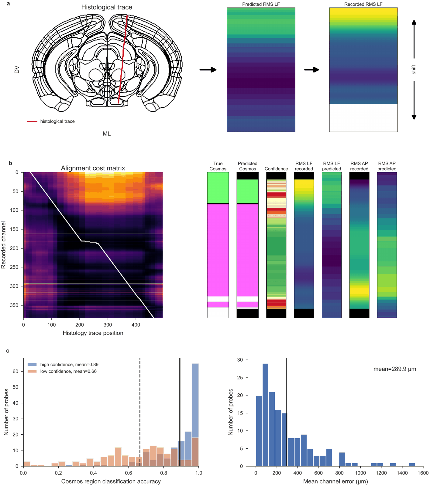
Alignment along the histology track: the spatial encoder’s predictions along the trace (a) are matched to the recorded features by dynamic time warping on a cost matrix (b); over held-out probes, confident alignments get most regions right (c).

The IBL alignment GUI runs the same alignment interactively, through its Channel Prediction plugin.

What this repository is not

ibleatools is the public inference package: feature computation plus loading and running published models. Training scripts and figure production live in paper-ephys-atlas, which calls this package, and a test (tests/test_repo_segregation.py) enforces the one-way dependency — importing the public surface must pull in nothing from examples/.

That is why every model here arrives as a published artifact with a manifest rather than as something you fit yourself.