How to plot region predictions along the probe
A region decoder returns one row per channel. Drawn against depth, beside the histology, those rows answer the question at a glance: where along the probe does the model agree with the anatomy, where does it hesitate, and between which regions?
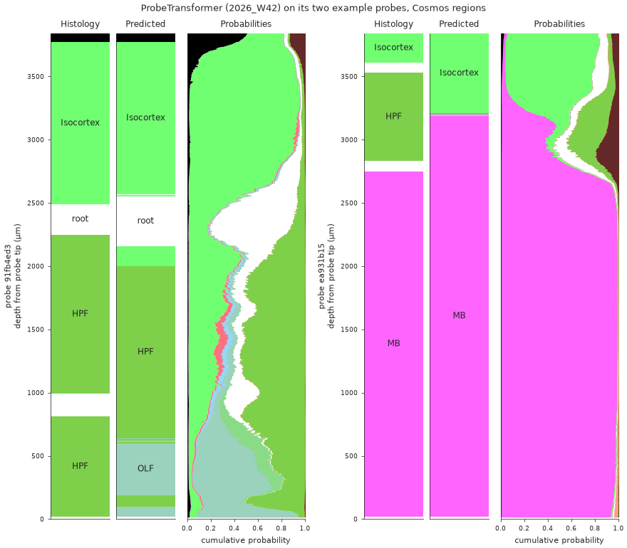
2026_W42) on the two probes bundled with it. For each probe, from left to right: the Cosmos regions from histology, the predicted region, and the full posterior as stacked bands. On 91fb4ed3 the prediction follows Isocortex, root and HPF but calls the bottom of the probe OLF. On ea931b15 it finds Isocortex and midbrain (MB), while the hippocampus (HPF) between them shows up only as a minority band of the posterior.The model and its example come from the Hugging Face Hub. The histology of the two example probes is open data in the IBL public database, read through ONE.
Predict
The whole-probe decoder ships an example of two complete probes, with axial_um, so it can be drawn along depth. (The XGBoost decoder’s example is 500 channels drawn from many probes, which cannot.)
import pandas as pd
from ephysatlas import load_pretrained

model = load_pretrained(
    "int-brain-lab/ea-decoder-channel-transformer", revision="2026_W42"
)
df = pd.read_parquet(model.path_model / "example" / "features_sample.parquet")
out = model.predict(df)
On your own probe, df is your aggregated and denoised table; see predict brain regions.
The histology to compare against
For an IBL insertion, the channel locations come with the spike sorting. SpikeSortingLoader.load_channels returns them, with axial_um and an Allen atlas_id per channel:
from brainbox.io.one import SpikeSortingLoader
from one.api import ONE

one = ONE(base_url="https://openalyx.internationalbrainlab.org",
          password="international", silent=True)

pid = "91fb4ed3-ee27-4d7e-ba5d-f61202ed9884"
channels = SpikeSortingLoader(pid=pid, one=one).load_channels()
On your own recording, the histology is your traced track: the GUI’s channel locations after alignment, or any table with axial_um and atlas_id.
Plot
figure_predictions_along_probe draws one probe in three panels: the histology, the predicted region and the class probabilities as stacked bands.
import ephysatlas.plots

# The depth of each predicted channel: the decoder drops channels with non-finite features
pred = out.loc[pid].join(df.loc[pid, "axial_um"])

fig, axs = ephysatlas.plots.figure_predictions_along_probe(
    pred,
    pred["axial_um"],
    model.config["classes"],             # one id per class, in the order of the p_ columns
    histology=channels,                  # axial_um and an Allen atlas_id per channel
    mapping=model.config["region_map"],  # draw the histology in the model's Cosmos regions
    show_legend=True,
)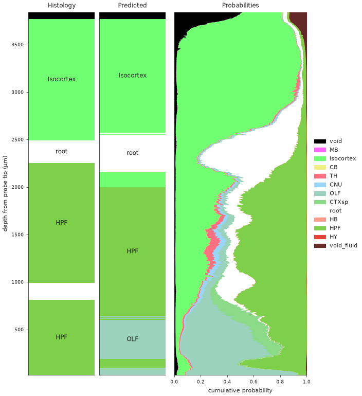
91fb4ed3: the Cosmos regions from histology, the predicted region, and the probabilities of the 13 classes as stacked bands. The prediction follows Isocortex, root and HPF, and calls the bottom of the probe OLF.The histology is mapped to the model’s region map, so both bars use the same 13 classes. The regions include the decoder’s extra void_fluid class (id 2000), which plain iblatlas BrainRegions does not know. If you pass your own regions, add that class with ClassifierRegions().add_new_region(NEW_VOID) from ephysatlas.anatomy, or its band is missing from the plot.
Each panel can be turned off (show_histology, show_prediction, show_probabilities), and so can the acronyms on the bars (show_labels). To put several probes on one figure, create the axes yourself and pass three per probe with axs=. examples/plot_predictions_along_probe.py draws the figure at the top of this page that way.
Reading it
- Where the bands are flat and one colour wins, the model is sure. A long run of one predicted region against the same histology region is a confirmed stretch of probe.
- Where two colours share the width, the channel is ambiguous between them. These are usually neighbouring regions, and the boundary between them is where alignment errors hide. The runner-up is the second-largest band.
- A region present in the histology but only as a thin band in the posterior (HPF on
ea931b15) is a region the decoder rarely gets right in isolation. The confusion matrix says which. prediction_probabilityandseed_agreement(fold_agreementfor the XGBoost decoder) are per-channel columns ofout: plot them as two more strips to see the confidence along depth.
In the alignment GUI
The IBL alignment GUI draws the same predictions, live, beside the histology regions it is aligning. Its Channel Prediction plugin runs the decoders on an ibleatools feature table and lists them, with cumulative versions, among the region plots.
For an IBL insertion, ephysatlas.reveal.AtlasReveal draws the decoder output beside the features and the histology in one figure, figure_02_classifier_results. It needs ONE access, and either your predictions (df_predictions=) or a local model directory (path_model=).
Next steps
- Which brain regions is my probe in? — the whole workflow, recording to aligned probe
- Predict brain regions — the decoders’ inputs and outputs
- Features along the probe — the features behind the predictions
figure_predictions_along_probeAPI andplot_cumulative_probasAPI