How to aggregate and denoise features

Computing features gives you one table per snippet. The published models are trained on one table per channel, aggregated across snippets and then denoised. This guide is the step in between. Without it, the model gets inputs unlike the ones it was trained on.

Why this step exists

The region decoder’s manifest names the table it expects:

from ephysatlas import load_pretrained

model = load_pretrained(
    "int-brain-lab/ea-decoder-channel-xgboost", revision="2026_W42"
)
print(model.index["inputs"]["table"])   # raw_ephys_features_denoised.pqt

raw_ephys_features_denoised.pqt — the denoised table. Three things happen on the way there:

Aggregation. A single snippet is a few seconds of recording. Per-channel feature estimates from one window are noisy, and some are unstable. Taking the per-channel median across several windows spread through the recording (the mean for spike_count) is what makes them usable, and it is what the training data did.
Denoising. Applied per probe, using channel labels, this suppresses per-channel outliers along the probe axis. Some features are also transformed here: rms_ap and rms_lf are denoised in dB and spike_count in log2, and they are returned in those transformed units. A model trained on denoised features therefore expects dB, not volts.
Waveform remap. Since ephysatlas 0.9.0 the six raw timing and amplitude waveform columns (peak_val, trough_val, peak_time_secs, trough_time_secs, tip_time_secs, recovery_time_secs) are replaced by four interpretable ones (spike_width_secs, predepolarisation_width_secs, spike_amplitude, peak_to_trough_ratio_log). The published 2026_W42 tables are remapped too.

Feeding a raw single-snippet table to the model is a units-and-distribution mismatch. The model still runs, but its predictions are wrong.

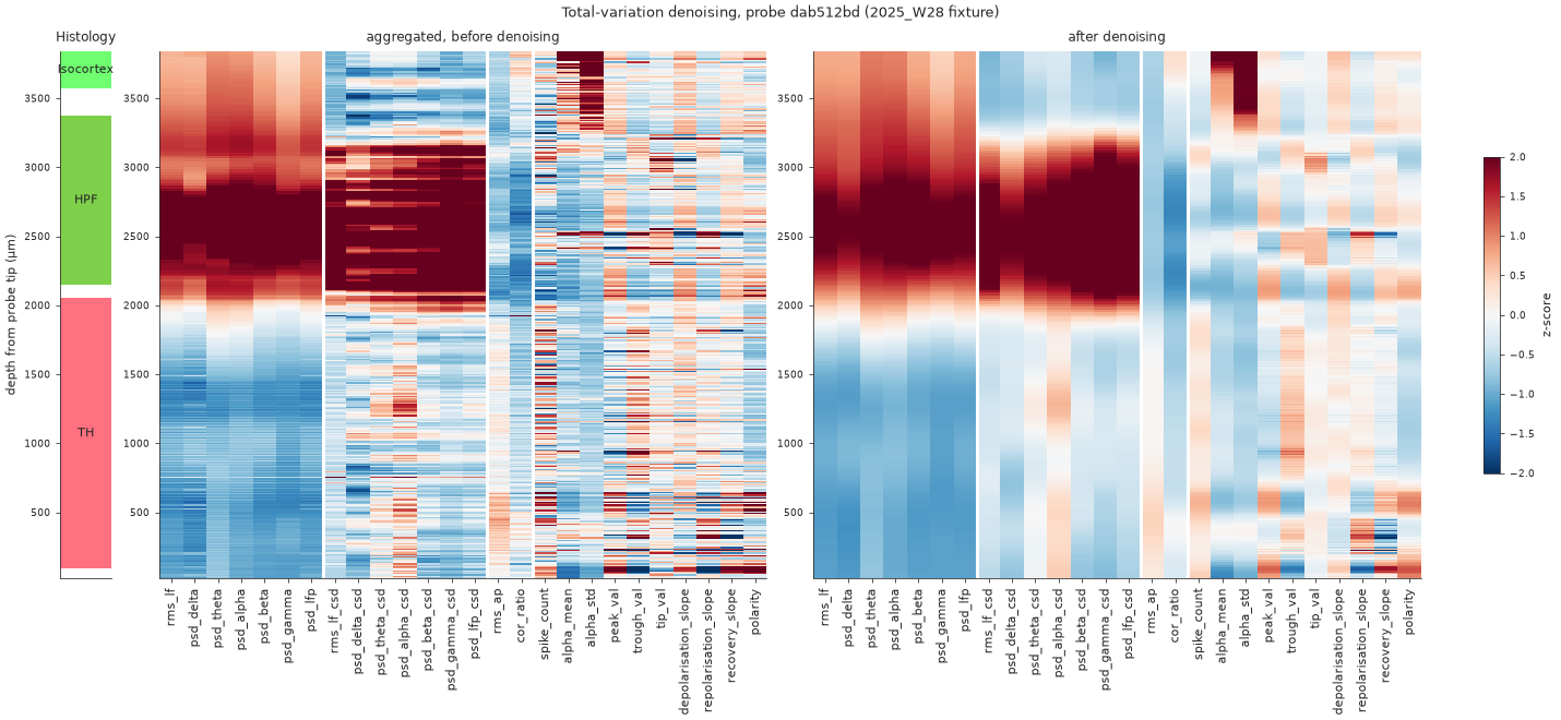
What denoising does to one probe of the committed 2025_W28 fixture: the aggregated table (left) and the denoised one (right), z-scored on one colour scale beside the histology. Channel-to-channel noise goes, region boundaries stay. Code. — What denoising does to one probe of the committed `2025_W28` fixture: the aggregated table (left) and the denoised one (right), z-scored on one colour scale beside the histology. Channel-to-channel noise goes, region boundaries stay. Code.

Prerequisites

Several snippets already computed to disk with output_dir set. See write the snippets yourself; that loop produces exactly what this page consumes. If you have not computed any snippets yet, skip to straight from a calculator.

Your output tree should look like this:

/data/features/
└── subject42_probe00/                                    ← probe_level_dir
    ├── channels.pqt
    ├── probe_subject42_probe00_000300.0_01.0_01.0/
    ├── probe_subject42_probe00_000900.0_01.0_01.0/
    ├── probe_subject42_probe00_001500.0_01.0_01.0/
    └── probe_subject42_probe00_002100.0_01.0_01.0/

The whole thing in one call

produce_output_dataframes orchestrates the entire pipeline: aggregate channel metadata, aggregate raw features, denoise, remap the waveform features:

from pathlib import Path

import ephysatlas.aggregation
import ephysatlas.utils

probe_level_dir = Path("/data/features/subject42_probe00")
input_dir = Path("/data/features")
output_dir = Path("/data/features/aggregated")

# One row per snippet, read from the provenance stamped on the feature files
snippets_df = ephysatlas.utils.get_aggregated_snippets_df(probe_level_dir)
print(snippets_df.shape)   # (4, n_metadata_columns) for the tree above

df_channels, df_raw, df_denoised = ephysatlas.aggregation.produce_output_dataframes(
    snippets_df, input_dir, output_dir
)

print(df_denoised.shape)         # (n_channels, n_features)
print(df_denoised.index.names)   # ['pid', 'channel']

With output_dir given, four files are written:

file	content
`snippets_df.pqt`	The input snippet table, for the record
`channels.pqt`	Aggregated channel metadata and positions
`raw_ephys_features.pqt`	Aggregated raw features
`raw_ephys_features_denoised.pqt`	Denoised features — a model’s input, once you add `outside` (below)

That mirrors the layout of the published IBL aggregates, so anything that reads those reads your output too.

Straight from a calculator

If the snippets are not on disk yet, a calculator’s compute_denoised_features does everything: it picks the windows, computes each snippet, then runs the same median, denoising and remap:

df_denoised = calc.compute_denoised_features(
    n_snippets=5, duration_ap=5.0, duration_lf=5.0
)
print(df_denoised.index.names)   # ['pid', 'channel'], with pid = calc.name

This works on every calculator (SpikeGLX, IBL, NWB, Zarr, LFPack, NumPy). The snippet files go to a temporary folder that is removed afterwards, unless you pass options with an output_dir. Nothing is written for the aggregate itself. Use produce_output_dataframes when you want the four files above. To choose the windows yourself, use compute_aggregated_features; see choose the snippet windows.

Several probes at once

snippets_df is keyed by pid, so aggregating many probes is one concatenation. Nothing in the pipeline assumes a single probe:

import pandas as pd

probe_dirs = [
    Path("/data/features/subject42_probe00"),
    Path("/data/features/subject42_probe01"),
    Path("/data/features/subject43_probe00"),
]

snippets_df = pd.concat(
    [ephysatlas.utils.get_aggregated_snippets_df(d) for d in probe_dirs],
    ignore_index=True,
)

df_channels, df_raw, df_denoised = ephysatlas.aggregation.produce_output_dataframes(
    snippets_df, Path("/data/features"), Path("/data/features/aggregated")
)

Denoising is applied per probe, so probes never contaminate each other regardless of how many you pass at once.

Running the steps separately

Use the individual functions when you want the intermediate table — to inspect the raw aggregate, or to denoise a table you already have:

import ephysatlas.aggregation

# snippets -> one row per (pid, channel)
df_raw = ephysatlas.aggregation.get_aggregated_raw_features(
    snippets_df, output_dir=output_dir
)

# aggregated raw -> denoised
df_denoised = ephysatlas.aggregation.denoise_raw_features_data(df_raw)

# raw waveform columns -> the spike-shape set, as produce_output_dataframes does
df_denoised = ephysatlas.aggregation.apply_waveform_remap(df_denoised)

Skip the last step and df_denoised keeps the six raw waveform columns, which the 2026_W42 models do not read.

Both parallelise over probes with joblib. n_jobs=-1 (the default) uses every processor; set n_jobs=1 when debugging, so tracebacks are readable, and verbose=0 to silence progress output.

Important

denoise_raw_features_data takes the bad channels from a channel_labels column on its input. It comes from the channel metadata that get_aggregated_raw_features merges in. A table without it, assembled by hand or from an LF-only source with no stored labels, logs a warning and has every channel labelled good (0), so bad channels are filtered like good ones instead of being interpolated over.

Add the one derived column a model needs

df_denoised still lacks outside, a boolean the models require. It is derived from the channel labels rather than stored, so add it before predicting:

df_denoised["outside"] = df_denoised["channel_labels"] == 3

read_features_from_disk does this for you, and the published df_all_cols_merged.pqt already contains it. But the table produce_output_dataframes writes does not, and neither does compute_denoised_features. Verified against the published ea_active/2026_W42 aggregate, whose raw_ephys_features_denoised.pqt carries 47 of the 2026_W42 decoder’s 48 required columns, missing exactly this one.

Check the result before predicting

Compare the table against the model’s declared input list:

from ephysatlas import load_pretrained

model = load_pretrained(
    "int-brain-lab/ea-decoder-channel-xgboost", revision="2026_W42"
)

required = set(model.inputs["features"])
missing = sorted(required - set(df_denoised.columns))
print(f"{len(missing)} of {len(required)} required features missing")
print(missing)

predict also raises a KeyError naming the missing columns. Possible causes:

['outside'] — the derived column above.
A whole block of names — a feature family you did not compute. The 2026_W42 decoder needs 48 columns spanning all four families — lf, csd, ap and waveforms — so a table computed with features_to_compute=["lf", "csd"] alone cannot satisfy it. Waveform features need the [full] extra.
peak_val, trough_val, peak_time_secs and the other raw waveform columns — an older model on a remapped table. Use the 2026_W42 model.
The seven *_bpr columns — a 2026_W42 model on a table computed before 0.10.0, whose first-difference columns are *_csd_diff1. Recompute the features.

Denoising a single probe directly

For one probe already loaded in memory, the underlying function is available directly:

import ephysatlas.features

df_denoised = ephysatlas.features.denoise_dataframe(
    df_pid, channel_labels=df_pid["channel_labels"].to_numpy()
)

denoise_raw_features_data is a parallel wrapper over exactly this, called once per probe. Use the wrapper unless you have a reason not to. Neither remaps the waveform columns; apply_waveform_remap does.

The denoising strength fac defaults to one factor per feature group, ephysatlas.features.DEFAULT_FAC: 0.1 for raw_ap, raw_lf and raw_lf_csd, and 3 for waveforms. Pass a scalar to apply one factor to every group, or a dict to override some groups (the others then default to 1). Changing it changes the features a model sees, so keep the default unless you are re-training.

Next steps

Predict brain regions — feed the denoised table to the decoder
Plot features along the probe
Core concepts — vintages, and why denoising changes units
Feature list reference
produce_output_dataframes API and compute_aggregated_features API