Plot audio spectrogtam

For a given session eid (ephys session), plot spectrogram of sound recorded via the microphone. Example of using soundfile to read in .flac file extensions

# Author: Gaelle Chapuis

from ibllib.io.extractors.training_audio import welchogram
import soundfile as sf
import numpy as np
import matplotlib.pyplot as plt
from one.api import ONE

eid = '4ecb5d24-f5cc-402c-be28-9d0f7cb14b3a'  # TEST EXAMPLE
one = ONE(base_url='https://openalyx.internationalbrainlab.org', silent=True)
# -- Get raw data
filename = one.load_dataset(eid, '_iblrig_micData.raw.flac', download_only=True)
with open(filename, 'rb') as f:
    wav, fs = sf.read(f)

# -- Compute spectrogram over first 2 minutes
t_idx = 120 * fs
tscale, fscale, W, detect = welchogram(fs, wav[:t_idx])

# -- Put data into single variable
TF = {}

TF['power'] = W.astype(np.single)
TF['frequencies'] = fscale[None, :].astype(np.single)
TF['onset_times'] = detect
TF['times_mic'] = tscale[:, None].astype(np.single)

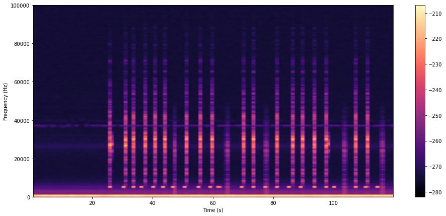
# # -- Plot spectrogram
tlims = TF['times_mic'][[0, -1]].flatten()
flims = TF['frequencies'][0, [0, -1]].flatten()
fig = plt.figure(figsize=[16, 7])
ax = plt.axes()
im = ax.imshow(20 * np.log10(TF['power'].T), aspect='auto', cmap=plt.get_cmap('magma'),
               extent=np.concatenate((tlims, flims)),
               origin='lower')
ax.set_xlabel(r'Time (s)')
ax.set_ylabel(r'Frequency (Hz)')
plt.colorbar(im)
plt.show()

 |████████████████████████████████████████████████████████████████████████████████████████████████████| 100.0%