Datajoint Introductory Tutorial
In this tutorial we will use datajoint to create a simple psychometric behavior plot.
This tutorial assumes that you have setup the unified ibl environment IBL python environment and set up your Datajoint credentials.
First let’s import datajoint
[1]:
import datajoint as dj
# for the purposes of tutorial limit the table print output to 5
dj.config['display.limit'] = 5
We can access datajoint tables by importing schemas from the IBL-pipeline. Let’s import the subject schema
[2]:
from ibl_pipeline import subject
Connecting mayofaulkner@datajoint.internationalbrainlab.org:3306
Within this schema there is a datajoint table called Subject. This holds all the information about subjects registered on Alyx under IBL projects. Let’s access this table and look at the first couple of entries
[3]:
subjects = subject.Subject()
subjects
Out[3]:
| subject_uuid | subject_nickname nickname | sex sex | subject_birth_date birth date | ear_mark ear mark | subject_line name | subject_source name of source | protocol_number protocol number | subject_description | subject_ts | subject_strain |
|---|---|---|---|---|---|---|---|---|---|---|
| 0026c82d-39e4-4c6b-acb3-303eb4b24f05 | IBL_32 | M | 2018-04-23 | None | C57BL/6NCrl | Charles River | 1 | None | 2019-08-06 21:30:42 | C57BL/6N |
| 00778394-c956-408d-8a6c-ca3b05a611d5 | KS019 | F | 2019-04-30 | None | C57BL/6J | None | 2 | None | 2019-08-13 17:07:33 | C57BL/6J |
| 00c60db3-74c3-4ee2-9df9-2c84acf84e92 | ibl_witten_10 | F | 2018-11-13 | notag | C57BL/6J | Jax | 3 | None | 2019-09-25 01:33:25 | C57BL/6J |
| 0124f697-16ce-4f59-b87c-e53fcb3a27ac | 6867 | M | 2018-06-25 | None | Thy1-GCaMP6s | CCU - Margarida colonies | 1 | None | 2019-09-25 01:33:25 | C57BL/6J |
| 019444e5-2192-4953-855d-084226fb965a | dop_48 | M | 2021-11-23 | 709 | Dat-Cre | Princeton | 2 | None | 2022-04-15 03:37:28 | C57BL/6J |
...
Total: 1318
Next, we will find the entry in the table for the same subject that we looked at in the ONE tutorial, KS022. To do this we will restrict the Subject table by the subject nickname
[4]:
subjects & 'subject_nickname = "KS022"'
Out[4]:
| subject_uuid | subject_nickname nickname | sex sex | subject_birth_date birth date | ear_mark ear mark | subject_line name | subject_source name of source | protocol_number protocol number | subject_description | subject_ts | subject_strain |
|---|---|---|---|---|---|---|---|---|---|---|
| b57c1934-f9d1-4dc4-a474-e2cb4acdf918 | KS022 | M | 2019-06-25 | None | C57BL/6J | None | 3 | None | 2019-09-20 04:28:14 | C57BL/6J |
Total: 1
We now want to find information about the behavioural sessions. This information is stored in a table Session defined in the acquisition schema. Let’s import this schema, access the table and display the first few entries
[5]:
from ibl_pipeline import acquisition
sessions = acquisition.Session()
sessions
Out[5]:
| subject_uuid | session_start_time start time | session_uuid | session_number number | session_end_time end time | session_lab name of lab | session_location name of the location | task_protocol | session_type type | session_narrative | session_ts |
|---|---|---|---|---|---|---|---|---|---|---|
| 00778394-c956-408d-8a6c-ca3b05a611d5 | 2019-08-07 10:49:41 | 0955e23e-90cf-4250-a092-82fabdf67a24 | 1 | 2019-08-07 11:23:14 | cortexlab | _iblrig_cortexlab_behavior_3 | _iblrig_tasks_habituationChoiceWorld5.2.5 | Experiment | None | 2019-08-13 17:26:00 |
| 00778394-c956-408d-8a6c-ca3b05a611d5 | 2019-08-08 15:32:40 | 996167fa-07bc-4afe-b7b9-4aee0ba75c1f | 1 | 2019-08-08 16:19:23 | cortexlab | _iblrig_cortexlab_behavior_3 | _iblrig_tasks_habituationChoiceWorld5.2.5 | Experiment | None | 2019-08-13 17:26:01 |
| 00778394-c956-408d-8a6c-ca3b05a611d5 | 2019-08-09 10:37:49 | 13e38e6c-0cd6-41f9-a2ab-8d6021fea035 | 1 | 2019-08-09 11:40:12 | cortexlab | _iblrig_cortexlab_behavior_3 | _iblrig_tasks_habituationChoiceWorld5.2.7 | Experiment | None | 2019-08-13 17:26:00 |
| 00778394-c956-408d-8a6c-ca3b05a611d5 | 2019-08-10 11:24:59 | fb9bdf18-76be-452b-ac4e-21d5de3a6f9f | 1 | 2019-08-10 12:11:04 | cortexlab | _iblrig_cortexlab_behavior_3 | _iblrig_tasks_trainingChoiceWorld5.2.7 | Experiment | None | 2019-08-13 17:26:06 |
| 00778394-c956-408d-8a6c-ca3b05a611d5 | 2019-08-12 09:21:03 | d47e9a4c-18dc-4d4d-991c-d30059ec2cbd | 1 | 2019-08-12 10:07:19 | cortexlab | _iblrig_cortexlab_behavior_3 | _iblrig_tasks_trainingChoiceWorld5.2.7 | Experiment | None | 2019-08-14 12:37:53 |
...
Total: 51591
If we look at the primary keys (columns with black headings) in the Subjects and Sessions table, we will notice that both contain subject_uuid as a primary key. This means that these two tables can be joined using *****.
We want to find information about all the sessions that KS022 did in the training phase of the IBL training pipeline. When combining the tables we will therefore restrict the Subject table by the subject nickname (as we did before) and the Sessions table by the task protocol
[6]:
(subjects & 'subject_nickname = "KS022"') * (sessions & 'task_protocol LIKE "%training%"')
Out[6]:
| subject_uuid | session_start_time start time | subject_nickname nickname | sex sex | subject_birth_date birth date | ear_mark ear mark | subject_line name | subject_source name of source | protocol_number protocol number | subject_description | subject_ts | subject_strain | session_uuid | session_number number | session_end_time end time | session_lab name of lab | session_location name of the location | task_protocol | session_type type | session_narrative | session_ts |
|---|---|---|---|---|---|---|---|---|---|---|---|---|---|---|---|---|---|---|---|---|
| b57c1934-f9d1-4dc4-a474-e2cb4acdf918 | 2019-09-23 13:43:40 | KS022 | M | 2019-06-25 | None | C57BL/6J | None | 3 | None | 2019-09-20 04:28:14 | C57BL/6J | 242ed7aa-6e02-4d55-b003-874b71357074 | 1 | 2019-09-23 14:28:22 | cortexlab | _iblrig_cortexlab_behavior_3 | _iblrig_tasks_trainingChoiceWorld5.3.0 | Experiment | None | 2019-09-24 04:51:41 |
| b57c1934-f9d1-4dc4-a474-e2cb4acdf918 | 2019-09-24 10:41:18 | KS022 | M | 2019-06-25 | None | C57BL/6J | None | 3 | None | 2019-09-20 04:28:14 | C57BL/6J | be7f7832-006f-4f79-8079-6dea549c90c0 | 1 | 2019-09-24 11:27:11 | cortexlab | _iblrig_cortexlab_behavior_3 | _iblrig_tasks_trainingChoiceWorld5.3.0 | Experiment | None | 2019-09-25 04:51:58 |
| b57c1934-f9d1-4dc4-a474-e2cb4acdf918 | 2019-09-25 09:37:26 | KS022 | M | 2019-06-25 | None | C57BL/6J | None | 3 | None | 2019-09-20 04:28:14 | C57BL/6J | c4f55950-26ac-4cb6-be38-57d9e604f5fc | 1 | 2019-09-25 10:23:20 | cortexlab | _iblrig_cortexlab_behavior_3 | _iblrig_tasks_trainingChoiceWorld5.3.0 | Experiment | None | 2019-09-26 04:53:06 |
| b57c1934-f9d1-4dc4-a474-e2cb4acdf918 | 2019-09-26 14:43:24 | KS022 | M | 2019-06-25 | None | C57BL/6J | None | 3 | None | 2019-09-20 04:28:14 | C57BL/6J | 39a0993b-ea91-4d7d-aa8b-84365ae77a81 | 1 | 2019-09-26 15:31:48 | cortexlab | _iblrig_cortexlab_behavior_3 | _iblrig_tasks_trainingChoiceWorld5.3.0 | Experiment | None | 2019-09-27 04:53:22 |
| b57c1934-f9d1-4dc4-a474-e2cb4acdf918 | 2019-09-27 10:21:16 | KS022 | M | 2019-06-25 | None | C57BL/6J | None | 3 | None | 2019-09-20 04:28:14 | C57BL/6J | f1eb053b-3cc2-45df-bbd5-2f5f54f05d23 | 1 | 2019-09-27 11:06:09 | cortexlab | _iblrig_cortexlab_behavior_3 | _iblrig_tasks_trainingChoiceWorld5.3.0 | Experiment | None | 2019-09-28 04:53:37 |
...
Total: 19
There is a lot of information in this table and we are not interested in all of it for the purposes of our analysis. Let’s just use the proj method to restrict the data presented. We do not want any columns from the Subject table (apart from the primary keys) and only want session_uuid from the Sesssions table. So we can write,
[7]:
((subjects & 'subject_nickname = "KS022"').proj() *
 (sessions & 'task_protocol LIKE "%training%"')).proj('session_uuid')
Out[7]:
| subject_uuid | session_start_time start time | session_uuid |
|---|---|---|
| b57c1934-f9d1-4dc4-a474-e2cb4acdf918 | 2019-09-23 13:43:40 | 242ed7aa-6e02-4d55-b003-874b71357074 |
| b57c1934-f9d1-4dc4-a474-e2cb4acdf918 | 2019-09-24 10:41:18 | be7f7832-006f-4f79-8079-6dea549c90c0 |
| b57c1934-f9d1-4dc4-a474-e2cb4acdf918 | 2019-09-25 09:37:26 | c4f55950-26ac-4cb6-be38-57d9e604f5fc |
| b57c1934-f9d1-4dc4-a474-e2cb4acdf918 | 2019-09-26 14:43:24 | 39a0993b-ea91-4d7d-aa8b-84365ae77a81 |
| b57c1934-f9d1-4dc4-a474-e2cb4acdf918 | 2019-09-27 10:21:16 | f1eb053b-3cc2-45df-bbd5-2f5f54f05d23 |
...
Total: 19
Note
In the above expression we first used proj and then joined the tables using ** * . We could have also joined the tables first and then usedproj**,
 ((subjects & 'subject_nickname = "KS022"') * (sessions & 'task_protocol LIKE "%training%"')
).proj('session_uuid')
Note that the session_uuid corresponds to the eID string in ONE.
Up until now we have been inspecting the content of the tables but do not actually have access to the content. This is because we have not actually read the data from the tables into memory yet. For this we would need to use the fetch command. Let’s fetch the session uuid information into a pandas dataframe
[8]:
eids = ((subjects & 'subject_nickname = "KS022"').proj() *
        (sessions & 'task_protocol LIKE "%training%"').proj('session_uuid')).fetch(format='frame')
[9]:
eids
Out[9]:
| session_uuid | ||
|---|---|---|
| subject_uuid | session_start_time | |
| b57c1934-f9d1-4dc4-a474-e2cb4acdf918 | 2019-09-23 13:43:40 | 242ed7aa-6e02-4d55-b003-874b71357074 |
| 2019-09-24 10:41:18 | be7f7832-006f-4f79-8079-6dea549c90c0 | |
| 2019-09-25 09:37:26 | c4f55950-26ac-4cb6-be38-57d9e604f5fc | |
| 2019-09-26 14:43:24 | 39a0993b-ea91-4d7d-aa8b-84365ae77a81 | |
| 2019-09-27 10:21:16 | f1eb053b-3cc2-45df-bbd5-2f5f54f05d23 | |
| 2019-10-01 11:01:44 | a07e255f-cf31-47aa-9667-5c62b93443e0 | |
| 2019-10-02 10:02:36 | fc7b7ea7-55c4-48fd-bb7b-2422c741fe8e | |
| 2019-10-03 14:15:32 | 22f33af3-5e77-4517-94b9-2cfefea27a10 | |
| 2019-10-04 10:52:19 | 7e508dce-e08c-4481-b634-1a9358673aa5 | |
| 2019-10-07 10:59:27 | 548ca39d-8898-460c-a930-785083b4127d | |
| 2019-10-08 11:19:34 | 3f815a05-a114-4a16-96ef-b398bd5a0b88 | |
| 2019-10-10 11:00:46 | f6c9daee-3e1e-4a5d-b372-7be8fcda5512 | |
| 2019-10-11 11:01:47 | 2f7e07d4-d713-46a1-8bce-6b497af405fc | |
| 2019-10-14 11:30:31 | 228b29b2-fb77-40c9-bd32-953fd5297896 | |
| 2019-10-15 10:32:56 | 9ee8bd6b-1e5e-4440-bc2e-7c001abe7b60 | |
| 2019-10-17 11:32:30 | 777ecfb9-616f-4ff9-a8d9-eb38f897a19f | |
| 2019-10-18 11:52:53 | 4e626e22-747e-4324-96f1-9827b7ca950d | |
| 2019-10-21 11:44:49 | dd4ad209-fcff-4252-9e38-44cba17f7603 | |
| 2019-10-22 11:48:05 | b4ac5904-5693-4d98-adb3-362e612836be |
Now that we have access to our list of session eIDs, we can get trial information associated with these sessions. The output from the trials dataset is stored in a table called PyschResults. We can import this from the analyses.behaviour schema
[10]:
from ibl_pipeline.analyses import behavior
trials = behavior.PsychResults()
trials
C:\Users\Mayo\iblenv\IBL-pipeline\ibl_pipeline\behavior.py:14: UserWarning: ONE not installed, cannot use populate
  warnings.warn('ONE not installed, cannot use populate')
Out[10]:
| subject_uuid | session_start_time start time | performance percentage correct in this session | performance_easy percentage correct of easy trials in this session | signed_contrasts contrasts used in this session, negative when on the left | n_trials_stim number of trials for each contrast | n_trials_stim_right number of reporting "right" trials for each contrast | prob_choose_right probability of choosing right, same size as contrasts | threshold | bias | lapse_low | lapse_high |
|---|---|---|---|---|---|---|---|---|---|---|---|
| 00778394-c956-408d-8a6c-ca3b05a611d5 | 2019-08-10 11:24:59 | 0.367347 | 0.367347 | =BLOB= | =BLOB= | =BLOB= | =BLOB= | 29.7063 | -58.2102 | 0.823603 | 0.409092 |
| 00778394-c956-408d-8a6c-ca3b05a611d5 | 2019-08-12 09:21:03 | 0.4 | 0.4 | =BLOB= | =BLOB= | =BLOB= | =BLOB= | 21.0607 | -58.2391 | 0.609229 | 0.181818 |
| 00778394-c956-408d-8a6c-ca3b05a611d5 | 2019-08-13 10:28:45 | 0.408072 | 0.408072 | =BLOB= | =BLOB= | =BLOB= | =BLOB= | 9.4945 | -0.13251 | 0.684564 | 0.364865 |
| 00778394-c956-408d-8a6c-ca3b05a611d5 | 2019-08-14 09:37:17 | 0.4 | 0.4 | =BLOB= | =BLOB= | =BLOB= | =BLOB= | 3.28746 | -67.9662 | 0.772727 | 0.454545 |
| 00778394-c956-408d-8a6c-ca3b05a611d5 | 2019-08-14 11:35:16 | 0.463668 | 0.463668 | =BLOB= | =BLOB= | =BLOB= | =BLOB= | 10.4665 | 99.3649 | 0.72314 | 0.0373897 |
...
Total: 41489
Let’s get the trial information for the first day KS022 trained. We will restrict the Sessions table by the day 1 eID and combine this with the trials table
[11]:
eid_day1 = dict(session_uuid=eids['session_uuid'][0])
trials_day1 = ((sessions & eid_day1).proj() * trials).fetch(format='frame')
trials_day1
Out[11]:
| performance | performance_easy | signed_contrasts | n_trials_stim | n_trials_stim_right | prob_choose_right | threshold | bias | lapse_low | lapse_high | ||
|---|---|---|---|---|---|---|---|---|---|---|---|
| subject_uuid | session_start_time | ||||||||||
| b57c1934-f9d1-4dc4-a474-e2cb4acdf918 | 2019-09-23 13:43:40 | 0.515432 | 0.515432 | [-1.0, -0.5, 0.5, 1.0] | [81, 90, 73, 80] | [41, 51, 50, 38] | [0.5061728395061729, 0.5666666666666667, 0.684... | 7.23087 | 86.8559 | 0.581967 | 0.525546 |
Notice how a lot of the metrics that we manually computed from the trials dataset in the previous ONE tutorial have already been computed for us and are available in the trials table. This is one advantage of Datajoint, common computations such as performance can be computed when the data is ingested and stored in tables.
We can find out which visual stimulus contrasts were presented to KS022 on day 1 and how many of each contrast by looking at the signed_contrasts and n_trials_stim attributes
[12]:
contrasts = trials_day1['signed_contrasts'].to_numpy()[0]
n_contrasts = trials_day1['n_trials_stim'].to_numpy()[0]
print(f"Visual stimulus contrasts on day 1 = {contrasts * 100}")
print(f"No. of each contrast on day 1 = {n_contrasts}")
Visual stimulus contrasts on day 1 = [-100.  -50.   50.  100.]
No. of each contrast on day 1 = [81 90 73 80]
We can easily extract the performance by typing
[13]:
print(f"Correct = { trials_day1['performance'].to_numpy()[0] * 100} %")
Correct = 51.5432 %
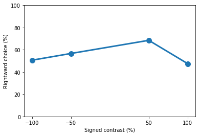
We can plot the peformance at each contrast by looking at the prob_choose_right attribute. The results stored in Datajoint are already expressed in terms of rightward choice, so we don’t need worry about converting any computations
[14]:
contrast_performance = trials_day1['prob_choose_right'].to_numpy()[0]

import matplotlib.pyplot as plt
plt.plot(contrasts * 100, contrast_performance * 100, 'o-', lw=3, ms=10)
plt.ylim([0, 100])
plt.xticks([*(contrasts * 100)])
plt.xlabel('Signed contrast (%)')
plt.ylabel('Rightward choice (%)')

print(contrast_performance)
[0.50617284 0.56666667 0.68493151 0.475 ]
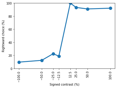
Let’s now repeat this for day 15 of training
[15]:
eid_day15 = dict(session_uuid=eids['session_uuid'][14])
trials_day15 = ((sessions & eid_day15).proj() * trials).fetch(format='frame')
contrasts = trials_day15['signed_contrasts'].to_numpy()[0]
n_contrasts = trials_day15['n_trials_stim'].to_numpy()[0]
print(f"Visual stimulus contrasts on day 1 = {contrasts * 100}")
print(f"No. of each contrast on day 1 = {n_contrasts}")
Visual stimulus contrasts on day 1 = [-100.   -50.   -25.   -12.5   12.5   25.    50.   100. ]
No. of each contrast on day 1 = [ 94  65 107  16  21  75  78  64]
[16]:
print(f"Correct = { trials_day15['performance'].to_numpy()[0] * 100} %")
Correct = 88.2692 %
[17]:
contrast_performance = trials_day15['prob_choose_right'].to_numpy()[0]

plt.plot(contrasts * 100, contrast_performance * 100, 'o-', lw=3, ms=10)
plt.ylim([0, 100])
plt.xticks([*(contrasts * 100)])
plt.xlabel('Signed contrast (%)')
plt.ylabel('Rightward choice (%)')
plt.xticks(rotation=90)

print(contrast_performance)
[0.09574468 0.12307692 0.22429907 0.1875     1.         0.93333333
 0.91025641 0.921875  ]
If we compare the results with the ONE tutorial, we will find that we have replicated those results using Datajoint, congratulations!
You should now be comfortable with the basics of exploring the Datajoint IBL pipeline. More Datajoint tutorials can be found in the IBL-Pipeline github or on the Datajoint jupyter.