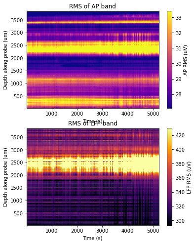
Download and plot RMS of raw data

Downloads rms data for a given session and probe and plots a heatmap of rms in AP and LFP band on the channels along probe for duration of ephys recording.

# import modules
from one.api import ONE
import matplotlib.pyplot as plt
import numpy as np

# instantiate ONE
one = ONE(base_url='https://openalyx.internationalbrainlab.org', silent=True)

# Specify subject, date and probe we are interested in
subject = 'CSHL049'
date = '2020-01-08'
sess_no = 1
probe_label = 'probe00'
eid = one.search(subject=subject, date=date, number=sess_no)[0]

# Download the data
# channels.rawInd: Index of good recording channels along probe
# channels.localCoordinates: Position of each recording channel along probe
channels = one.load_object(eid, 'channels', collection=f'alf/{probe_label}')

# Get range for y-axis
depth_range = [np.min(channels.localCoordinates[:, 1]),
               np.max(channels.localCoordinates[:, 1])]

# RMS data associated with AP band of data
rms_ap = one.load_object(eid, 'ephysTimeRmsAP', collection=f'raw_ephys_data/{probe_label}')
rms_ap_data = rms_ap['rms'][:, channels.rawInd] * 1e6  # convert to uV

# Median subtract to clean up the data
median = np.mean(np.apply_along_axis(lambda x: np.median(x), 1, rms_ap_data))
# Add back the median so that the actual values in uV remain correct
rms_ap_data_median = np.apply_along_axis(lambda x: x - np.median(x), 1, rms_ap_data) + median

# Get levels for colour bar and x-axis
ap_levels = np.quantile(rms_ap_data_median, [0.1, 0.9])
ap_time_range = [rms_ap['timestamps'][0], rms_ap['timestamps'][-1]]

# RMS data associated with LFP band of data
rms_lf = one.load_object(eid, 'ephysTimeRmsLF', collection=f'raw_ephys_data/{probe_label}')
rms_lf_data = rms_lf['rms'][:, channels.rawInd] * 1e6  # convert to uV
# Median subtract to clean up the data
median = np.mean(np.apply_along_axis(lambda x: np.median(x), 1, rms_lf_data))
rms_lf_data_median = np.apply_along_axis(lambda x: x - np.median(x), 1, rms_lf_data) + median

lf_levels = np.quantile(rms_lf_data_median, [0.1, 0.9])
lf_time_range = [rms_lf['timestamps'][0], rms_lf['timestamps'][-1]]

# Create figure
fig, ax = plt.subplots(2, 1, figsize=(6, 8))
# Plot the AP rms data
ax0 = ax[0]
rms_ap_plot = ax0.imshow(rms_ap_data_median.T, extent=np.r_[ap_time_range, depth_range],
                         cmap='plasma', vmin=ap_levels[0], vmax=ap_levels[1], origin='lower')
cbar_ap = fig.colorbar(rms_ap_plot, ax=ax0)
cbar_ap.set_label('AP RMS (uV)')
ax0.set_xlabel('Time (s)')
ax0.set_ylabel('Depth along probe (um)')
ax0.set_title('RMS of AP band')

# Plot the LFP rms data
ax1 = ax[1]
rms_lf_plot = ax1.imshow(rms_lf_data_median.T, extent=np.r_[lf_time_range, depth_range],
                         cmap='inferno', vmin=lf_levels[0], vmax=lf_levels[1], origin='lower')
cbar_lf = fig.colorbar(rms_lf_plot, ax=ax1)
cbar_lf.set_label('LFP RMS (uV)')
ax1.set_xlabel('Time (s)')
ax1.set_ylabel('Depth along probe (um)')
ax1.set_title('RMS of LFP band')

# Make sure it plots
plt.show()