Loading Spike Waveforms

Loading the spike sorting and average waveforms

%%capture
from one.api import ONE
from brainbox.io.one import SpikeSortingLoader

one = ONE(base_url='https://openalyx.internationalbrainlab.org')

pid = 'da8dfec1-d265-44e8-84ce-6ae9c109b8bd'

# Load in the spikesorting
ssl = SpikeSortingLoader(pid=pid, one=one)
spikes, clusters, channels = ssl.load_spike_sorting(revision='2024-05-06')
clusters = ssl.merge_clusters(spikes, clusters, channels)
waveforms = ssl.load_spike_sorting_object('waveforms')

Displaying a few average waveforms

import matplotlib.pyplot as plt
import numpy as np
import ibldsp.waveforms
from ibl_style.style import figure_style
figure_style()

cids = np.random.choice(np.where(clusters['label'] == 1)[0], 3)
fig, axs = plt.subplots(1, 3, figsize=(12, 4))
for i, cid in enumerate(cids):
    wf = waveforms['templates'][cid, :, :]
    ax = ibldsp.waveforms.double_wiggle(wf * 1e6 / 80, fs=30_000, ax=axs[i])
    ax.set(title=f'Cluster {cid}')

More details

During spike sorting, pre-processing operations are performed on the voltage data to create the average templates. Although those templates are useful for clustering, they may not be the best description of the neural activity. As such we extract average waveforms for each cluster using a different pre-processing. Details are provided on the spike sorting white paper on figshare. * Description of datasets

Exploring the raw waveforms

For each unit, we compiled up to raw data 256 waveforms chosen randomly from the entire recording. The pre-processing steps included rephasing of the channels, low-cut filtering, bad channel detection and common-average referencing.

To perform the loading we will use a convenience.

Warning, this will download a few Gigabytes of data to your computer !

Compute average waveform for cluster

Here we will load data from one cluster belonging to the striatum and compute the average waveform.

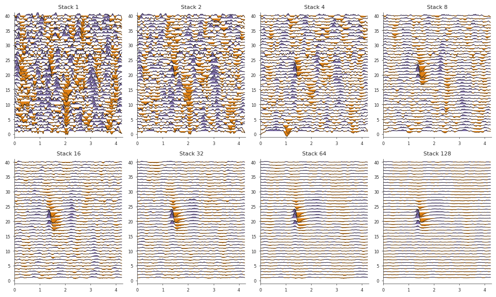
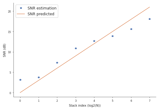
We will do so for several stack orders: 1, 2, 4, 8, 16, 32, 64, 128 and display the resulting waveform, while tracking the signal-to-noise ratio (SNR) for each stack order.

from ibldsp.utils import rms
# instantiating the waveform loader will download the raw waveform arrays and can take a few minutes (~3Gb)
wfl = ssl.raw_waveforms()
ic = np.where(np.logical_and(clusters['acronym'] == 'LSr', clusters['bitwise_fail'] == 0))[0]
# look at templates

raw_wav, info, channel_map = wfl.load_waveforms(labels=ic[12])

snr = np.zeros(8)
fig, axs = plt.subplots(2, 4, figsize=(10, 6))
for i, ax in enumerate(axs.flat):
    w_stack = np.mean(raw_wav[0, :(2 ** i), :, :], axis=0)
    ax = ibldsp.waveforms.double_wiggle( w_stack  * 1e6 / 80, fs=30_000, ax=axs.flatten()[i])
    ax.set_title(f"Stack {2 ** i}")
    snr[i] = 20 * np.log10(rms(w_stack[19:22, wfl.trough_offset - 10:wfl.trough_offset + 10].flatten()) / np.mean(rms(w_stack)))

100%|██████████| 12/12.0 [00:03<00:00,  3.00it/s]

For constant gaussian noise in n repeated experiments, we expect the SNR to scale proportionally to the square root of n. In decibels, this corresponds to 3dB / octave. Let’s see how the data compares to the prediction:

fig, ax = plt.subplots(figsize=(6, 4))
ax.plot(np.arange(8), snr, '*', label='SNR estimation')
ax.plot(np.arange(8), np.arange(8) * 3, label='SNR predicted')
ax.set(xlabel='Stack index (log2(N))', ylabel='SNR (dB)')
ax.legend()

<matplotlib.legend.Legend at 0x7b68b9b9a6d0>