Your first alignment

In this tutorial you will align a single-shank Neuropixels probe from the sample data. You will match three features in the electrophysiology to the brain regions along the probe’s track, save the result, and load it again.

Before you start

• Install the GUI (see Installation) and activate its virtual environment.

• Download the sample data and extract it. You will use the Sample data 1 folder: a single-shank Neuropixels 1.0 (3B) probe with 384 channels.

1. Open the sample data

1. Start the GUI:

   alignment-gui
   

   A window with empty plots opens.

2. Click the ... button in the top right corner and choose Open data folder….

3. Choose the Sample data 1 folder.

The data loads, and the four figures fill in:

• the Ephys figure on the left, with the electrophysiology along the probe

• the Histology figure, with the brain regions along the traced track

• the Slice figure, with a slice of the brain along the track

• the Fit figure, which will show how the track is stretched as you align

You will look at each figure as you need it. All of them are described in Interface.

The sample data comes with an alignment made on 7 October 2021, and the GUI starts from it: its reference line pair is drawn in the Ephys and Histology figures. You will make your own, so start from scratch:

4. Open the alignment dropdown in the top right corner. It lists 2021-10-07T08:19:16 and original.

5. Choose original.

The reference lines disappear, and the regions in the Histology figure are where the traced track alone puts them.

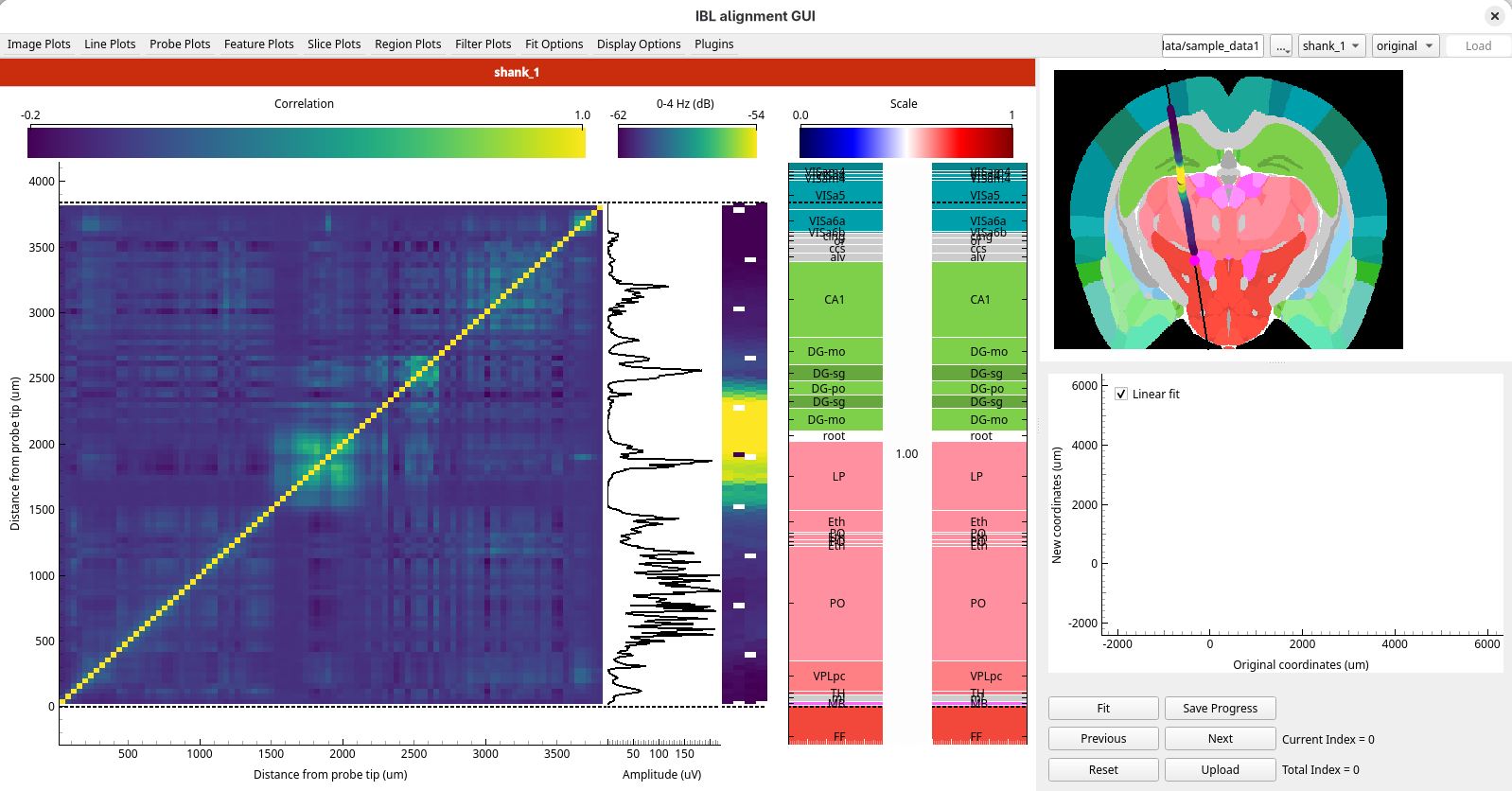
2. Get your bearings

Before placing any lines, look through the plots to get an overview of the features in the recording. Each panel of the Ephys figure has several plots, and a keyboard shortcut cycles through them:

• Alt+1 cycles through the image plots

• Alt+2 cycles through the line plots

• Alt+3 cycles through the probe plots

Press each one a few times to see what is available. Three features stand out in this recording.

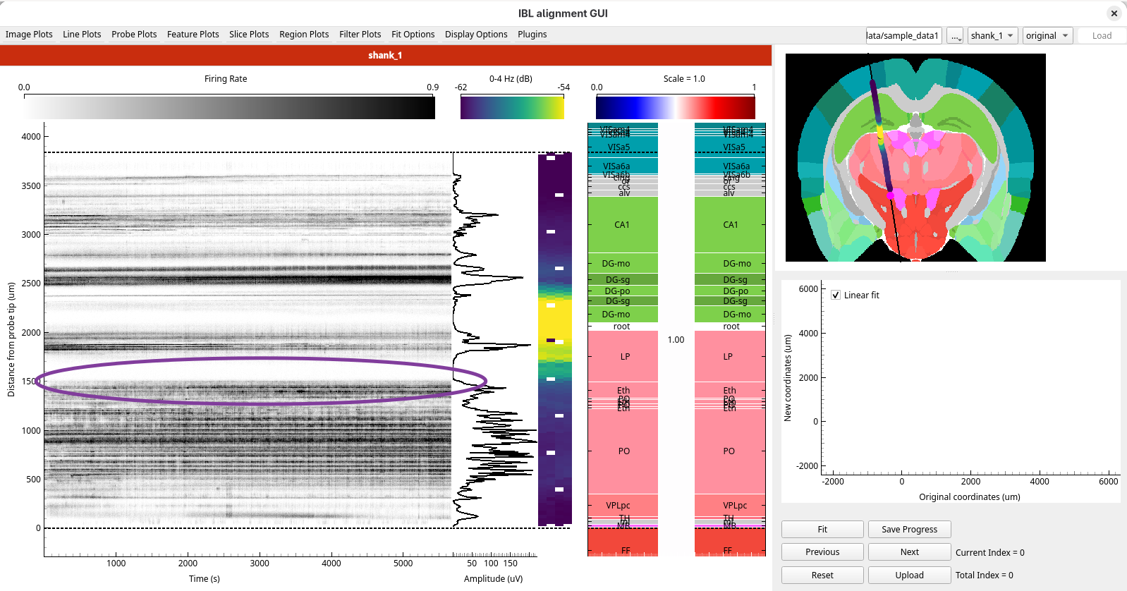
Firing rate

Select Firing Rate from the Image Plots menu. At around 1500 µm the pattern of firing changes: below it the firing rate is high, and above it there is a quiet stretch with little activity.

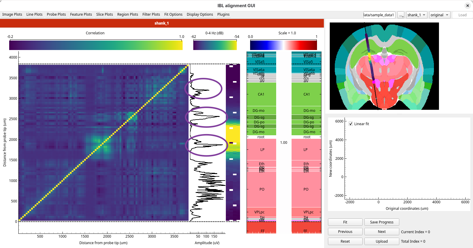
Amplitude

Select Amplitude from the Line Plots menu. It has three distinct peaks: one at around 1800 µm, one at around 2600 µm and one at around 3200 µm.

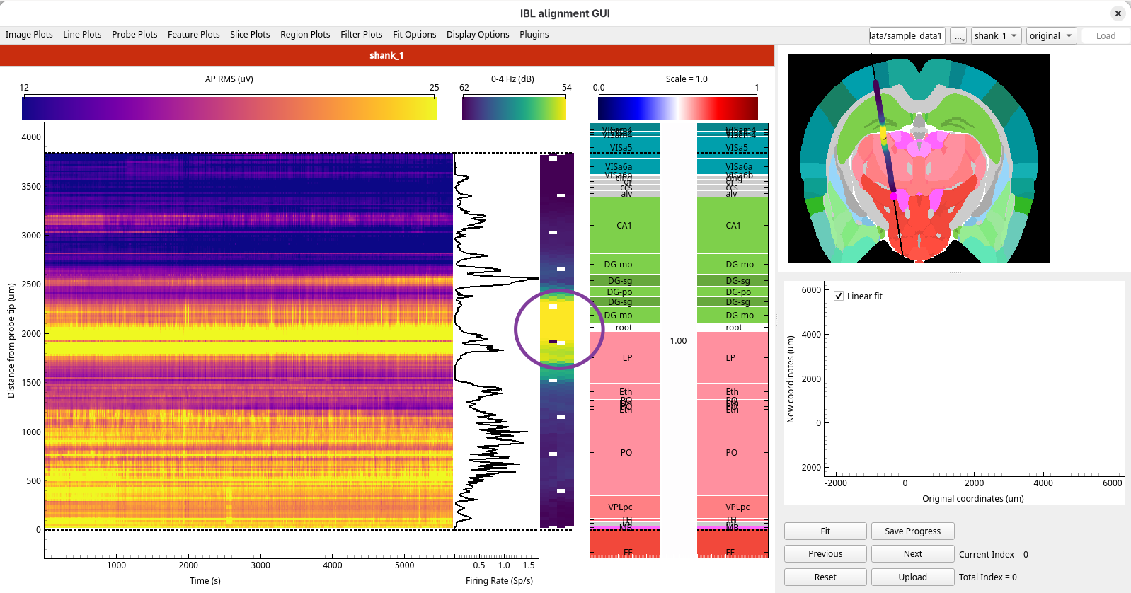
LFP power

Select 0 - 4 Hz from the Probe Plots menu. Between about 1800 µm and 2400 µm there is an area of high LFP power.

3. Add your first reference line pair

The first landmark we will look at is the change in firing pattern you saw in the Firing Rate image plot, at around 1500 µm. The high firing rate below it is likely to be in the thalamus, so this change probably marks the top of the thalamus. In the Histology figure, the thalamus is the salmon pink area.

1. Select Firing Rate from the Image Plots menu, if it is not still showing.

2. Double-click in the Ephys figure at around 1500 µm.

   A pair of lines appears: one in the Ephys figure and one in the Histology figure, in the same colour.

3. Drag the line in the Ephys figure onto the change in firing pattern, where the high firing rate below gives way to the quiet stretch above.

4. Drag the line in the Histology figure onto the top of the thalamus, the upper edge of the salmon pink area.

5. Press Enter, or click the Fit button below the Fit figure, to apply the fit.

The regions in the left panel of the Histology figure shift so that the boundary lines up with the feature. The channels in the Slice figure move along the track to match, and a point appears in the Fit figure.

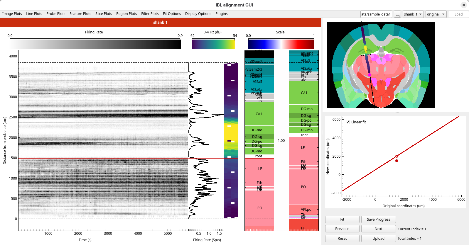
With one pair, the whole track is shifted by the same amount. Nothing is stretched yet.

4. Add a second pair

The second landmark we will consider is the amplitude peak at around 2600 µm in the Amplitude line plot. CA1, in the hippocampus, has a layer of large pyramidal neurons that can give spikes of high amplitude, so this peak is most likely in CA1. A layer inside a region has no boundary to line up with, so this time you align to roughly the centre of CA1.

1. Select Amplitude from the Line Plots menu, if it is not still showing.

2. Double-click in the Ephys figure at around 2600 µm to add a second pair.

3. Drag the line in the Ephys figure onto the amplitude peak.

4. Drag the line in the Histology figure to roughly the centre of CA1.

5. Press Enter or click Fit.

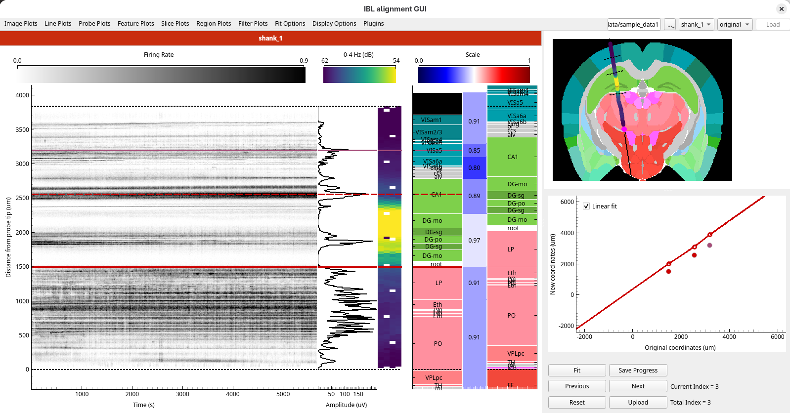
The track between your two lines is now stretched or compressed to fit both. Look at the middle panel of the Histology figure: it shows the scale factor between the lines, both by its colour and as a value. A scale factor above 1 means the regions there have been stretched to fit the electrophysiology, and below 1 that they have been compressed.

5. Add a third pair

The third landmark we will consider is the amplitude peak at around 3200 µm in the Amplitude line plot. Like CA1, layer 5 of the cortex has large pyramidal neurons that can give spikes of high amplitude, so this peak is likely to be in or near layer 5.

1. Double-click in the Ephys figure at around 3200 µm to add a third pair.

2. Drag the line in the Ephys figure onto the amplitude peak.

3. Drag the line in the Histology figure to roughly the centre of layer 5, as a best estimate.

4. Press Enter or click Fit.

The result is your three reference line pairs, with the regions in the Histology figure scaled to match them:

6. Understanding the fit

The Fit figure shows how your reference lines move the track. Each point is a reference line pair, plotted at its position along the track before the alignment and after it. The solid line is the fit that moves the regions:

• Between neighbouring reference lines, each stretch of the track is scaled separately, so the solid line is straight between points but can change slope at each one.

• Beyond your outermost lines there are no points to follow. With three or more pairs, a straight line is fitted through all the pairs, and the track beyond the outermost lines is scaled along it. This is the dotted line in the Fit figure, which appears once you add the third pair.

To see what the linear fit does:

1. Untick Linear fit in the top left corner of the Fit figure. The fit is applied again straight away.

2. Look at the Fit figure below your first point. The solid line no longer follows the dotted line: beyond the outermost lines, the regions are now only shifted, by the same amount as the nearest reference line, and not scaled.

3. Look at the regions below your first line and above your third line in the Histology figure, and at the scale factor in its middle panel.

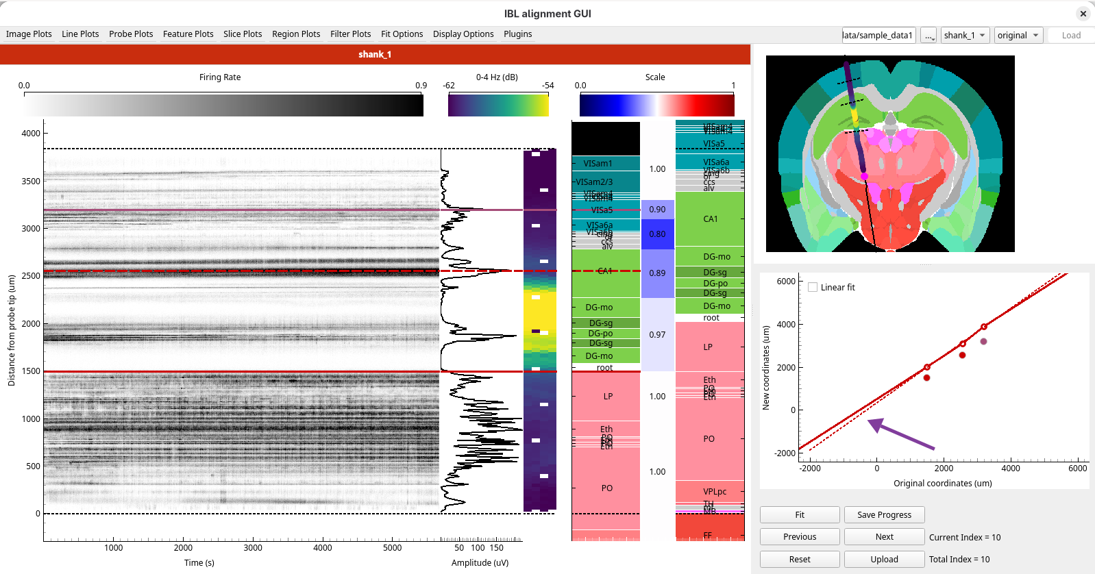
Tick Linear fit again before you go on. How alignment works explains the fit in more detail.

7. Check your alignment

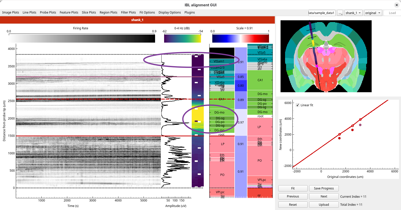
The three reference pairs used only two of the plots. Before going further, check the other features against what you would expect from the regions they now line up with. If they agree, your reference lines are probably reasonable. If they don’t, look again at the lines you placed.

1. Select 0 - 4 Hz from the Probe Plots menu. The area of high LFP power between about 1800 µm and 2400 µm should now line up with the dentate gyrus, which is expected to have high LFP power.

2. Select Firing Rate from the Image Plots menu. The firing disappears above about 3600 µm, which suggests the top of the probe may be outside the brain. In the Histology figure, the top of the probe has been assigned to the void, the black area outside the brain, which is consistent with this.

8. Step through your fits

1. Press Shift+Left, or click Previous, a few times. Each press goes back one fit, until the display shows your first fit with a single reference line pair.

2. Press Shift+Right, or click Next, until you are back at the latest one.

The Current Index label below the figures shows which fit you are on. Stepping back and forth like this is a quick way to compare two alignments.

9. Save your progress

Press Shift+S or click Save Progress. A file called alignment_progress.json appears in the Sample data 1 folder. If the GUI closed now, this alignment would be loaded again the next time you open the folder.

10. Upload the alignment

1. Press Shift+U or click Upload, then click Yes.

2. Open the Sample data 1 folder. Two files have been updated:

   • channel_locations.json now holds the position and brain region of every channel from your alignment

   • prev_alignments.json now holds your alignment as well as the 2021 one, so either can be loaded again

3. Open channel_locations.json and look at channel_0: its x, y and z are its position in µm relative to bregma, and brain_region is the region it is in.

alignment_progress.json has gone: uploading replaces the saved progress.

11. Load your alignment again

1. Choose Open data folder… again, and choose the Sample data 1 folder.

2. Look at the alignment dropdown in the top right corner. It lists your alignment, labelled with the date and time you uploaded it, then the 2021 alignment, then original. Yours is the most recent, so it is selected, and your reference lines are back.

3. Choose 2021-10-07T08:19:16. Its single reference line pair replaces yours. Compare where it puts the regions with where yours does.

4. Choose your alignment again.

What you’ve learned

You have:

• found features in the electrophysiology and matched them to region boundaries

• seen how one, two and three reference line pairs shift and stretch the track

• checked the alignment against features you did not use to place it

• saved work in progress, uploaded an alignment, and loaded it again

Next steps

• Aligning a multi-shank probe with a second recording: align a four-shank probe, with the help of a second recording

• How alignment works: what the fit does with your reference lines