Interface

This page describes the main window and what each part of it shows. Every menu entry is listed in Menus, and keyboard shortcuts in Keyboard shortcuts.

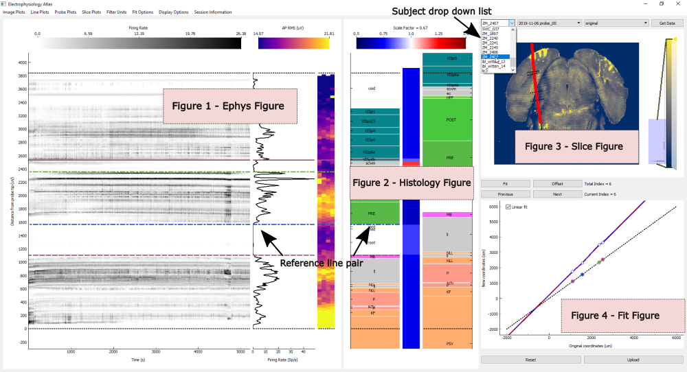
The window holds four figures. The data source button (...) in the top right corner opens a session (see How to open a session), and the alignment dropdown next to it chooses the saved alignment the active shank starts from (see How to continue from a previous alignment).

Zoom into the Ephys, Histology and Slice figures with the mouse wheel for a closer look. Press Shift+A to reset the axes of every figure.

Ephys figure

Electrophysiology data along the probe.

Image plots

2D data, as images or scatter plots. Switched from the Image Plots menu.

Line plots

1D data, as a line along the depth of the probe. Switched from the Line Plots menu.

Probe plots

2D data drawn on the probe geometry. Switched from the Probe Plots menu.

With the ephysatlas extra installed (see Optional dependencies) and a session with features, an extra panel can be added:

Prediction panel

A channel prediction, shown after the probe plot (or after the feature plot, in the feature view) once one is chosen from the Prediction Plots menu. Predictions are placed by depth along the probe, like the other ephys plots. The panel carries the reference lines, and its predicted regions are labelled with their acronyms. Choosing None removes it.

All predictions (side by side) (Shift+P) replaces the image, line and probe plots with one panel per prediction, to compare the models. Choosing any other plot returns to the usual view.

By default every unit from the spike sorting is shown. The Filter Plots menu restricts the plots to a class of units; which filters are available depends on the fields in clusters.metrics (see Input datasets).

Histology figure

The brain regions along the traced probe track, in three panels from left to right:

Scaled brain regions

The regions after the current alignment has been applied.

Scale factor

The scaling applied to each region along the track, shown both by its colour and as a value. Above 1 the region has been stretched, below 1 compressed (see How alignment works).

Original brain regions

The regions before any alignment.

Black dotted lines in the left and right panels mark the deepest and the shallowest channel.

The regions in all three panels can be shown with three mappings, chosen from the Set Mapping menu (see Brain region mappings). The 3D view and the uploaded results always use the Allen regions.

Allen

The full Allen atlas hierarchy.

Beryl

Allen regions grouped into larger areas.

Cosmos

The coarsest grouping, into a small number of major areas.

Slice figure

A slice through the brain along the traced trajectory. Each row of the image is taken from the trajectory coordinate at that depth, so a trajectory that is not smooth makes the image appear to jump between slices.

Overlaid on the slice:

• a black line through the traced points, extended to the top and bottom of the brain

• the channels along the trajectory, coloured by the plot shown in the Probe plots panel

• the reference lines, as black dotted lines perpendicular to the trajectory

The intensity of the image is set with the scale bar on the right of the figure.

The image is chosen from the Slice Plots menu:

• CCF: the Allen atlas average template (always available)

• Annotation: the Allen atlas annotation (always available)

• Histology red and Histology green: one entry per histology volume found for the session (see Input datasets)

Fit figure

The scaling applied along the depth of the trajectory.

Fit line

The piecewise fit along the trajectory. The points mark the reference lines.

Linear fit line (dotted)

A linear fit through all the reference lines. Shown when there are three or more.

The Linear fit checkbox in the top left corner of the figure sets whether the regions beyond the outermost reference lines are scaled by the linear fit. When it is unticked they are only offset.

With more than one shank in the grid layout, the Fit figure shows the fit of every shank.

After each fit, and after moving through the fits with Previous and Next, the coordinates of the reference line pairs are printed in the terminal, in µm: their depth along the probe (the original coordinates), along the track (the new coordinates), and the offset between them. These are the points of the Fit figure, more precisely than the figure can show.

Buttons

Fit

Apply the fit (Enter).

Next / Previous

Move through the last 10 fits (Shift+Right / Shift+Left).

Reset

Return the active shank to the alignment it was loaded with (Shift+R).

Upload

Save the alignment (see Output files) (Shift+U).

Save Progress

Save the alignment without uploading it, to recover it later (Shift+S).

Multiple shanks

When a session has more than one shank, or more than one configuration:

• In the tabbed layout each shank has its own tab. In the grid layout all shanks are shown at once. Switch between them with T.

• Change the active shank with Left and Right, or by clicking its tab in the tabbed layout.

• The active shank’s title is shown in red.

• Uploading asks which shanks to upload.