Predicting brain regions from the electrophysiology

In this tutorial you will use three different channel prediction models on the probe from Your first alignment, to predict the brain region of each channel from the electrophysiology. You will compare their predictions with the histology and with each other, and use them to place your own reference lines.

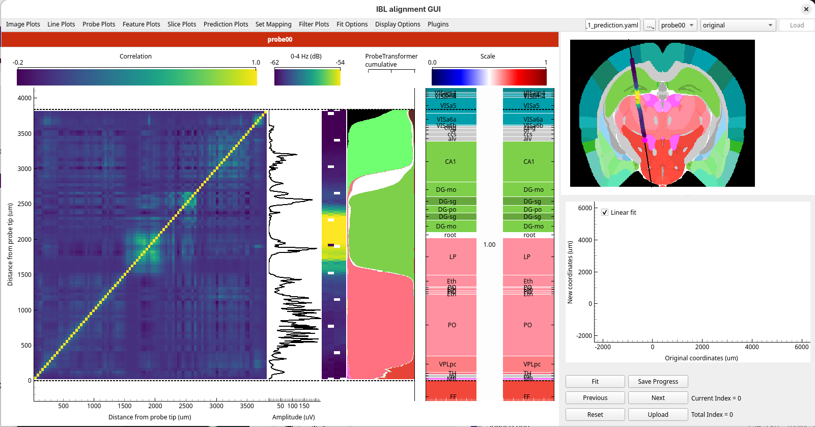
The models are downloaded the first time you use them, which can take a few minutes.

Before you start

• Complete Your first alignment.

• Install the ephysatlas extra (see How to install the optional extras). It also installs torch, which the alignment model needs.

• Find the sample_data_1_prediction folder in the sample data you extracted for Your first alignment, next to the sample_data_1 folder. It holds:

  • ephys_atlas_features_2026_W42.pqt: the electrophysiology features of every channel of Sample data 1, computed from the raw data with ibleatools

  • sample_data_1_prediction.yaml: a session YAML that loads Sample data 1 with these features

1. Check the plugin is installed

1. Start the GUI with alignment-gui.

2. Open the Plugins menu. It has a Channel Prediction entry, greyed out until you load a session with features in the next step.

If you do not see Channel Prediction as an option, the ephysatlas extra is not installed in the environment you started the GUI from.

2. Load the data with its features

The features are given to the GUI in a session YAML, alongside the data you opened in Your first alignment.

1. Open sample_data_1_prediction.yaml in a text editor:

   path: /path/to/ephys_alignment_sample_data
   
   probes:
     probe00:
       datasets:
         # The recording, histology and alignments of Sample data 1
         spike_sorting:
           path: sample_data_1
         histology:
           path: sample_data_1
         output:
           path: sample_data_1
         # The features the models run on
         features:
           path: sample_data_1_prediction/ephys_atlas_features_2026_W42.pqt
   

2. Set path to the full path of the folder that holds sample_data_1 and sample_data_1_prediction, and save the file.

   The other paths are relative to it. The spike sorting and histology come from sample_data_1, and the trajectory and the RMS and power spectra are read from there too, because they are saved beside the spike sorting. The results are written to sample_data_1 as well, so you carry on from your alignment in Your first alignment. Only the features come from sample_data_1_prediction.

3. In the GUI, click ..., choose Open session YAML…, and choose sample_data_1_prediction.yaml.

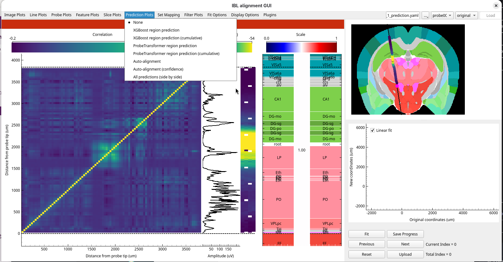
The data loads as before, and your alignment from Your first alignment is selected in the alignment dropdown. With the features loaded, the Feature Plots and Prediction Plots menus and Plugins → Channel Prediction are now available.

3. Look at the features

1. Open the Feature Plots menu and choose Ephys Atlas. The ephys plots are replaced by every feature side by side, each normalised along the probe.

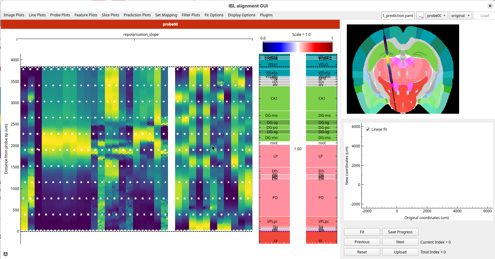
2. Look at where the features change along the probe. Many of them change together at the reference lines of your alignment from Your first alignment: at the top of the thalamus, at about 1500 µm, and at the top of CA1, at about 2700 µm.

These are the numbers the models work from: the same kinds of signal you looked at by eye in Your first alignment, computed for every channel. Choose any image plot to go back to the ephys plots.

4. Predict the regions with the region decoders

The first two models are region decoders: they predict the region of each channel directly from its electrophysiology features.

1. Choose original from the alignment dropdown, so the histology shows the track before any alignment.

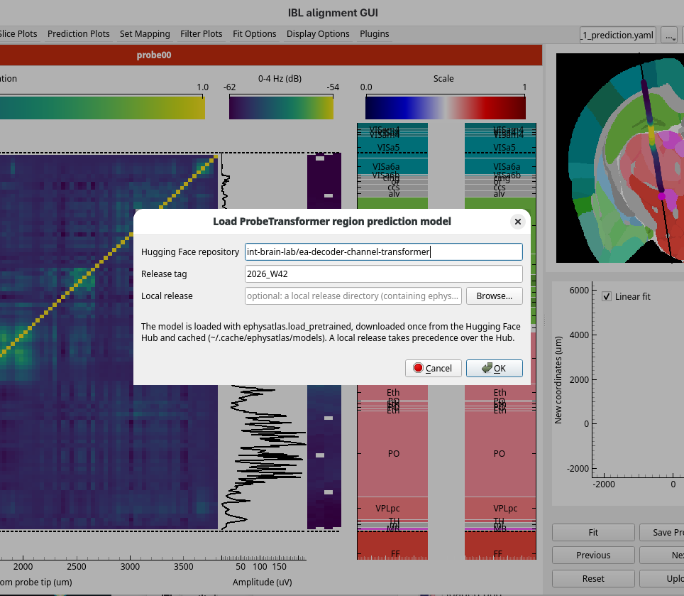
2. Open the Prediction Plots menu and choose ProbeTransformer region prediction.

3. The model’s dialog opens. Keep the default repository and release, and click OK. The model is downloaded the first time, then the prediction runs.

A panel titled ProbeTransformer prediction appears beside the ephys plots, showing the region the model predicts for each channel from the electrophysiology alone. Each predicted region is labelled with its acronym.

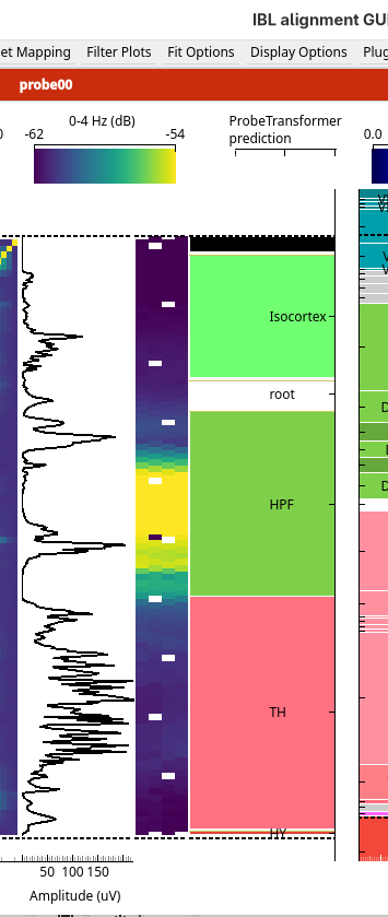
4. Compare the prediction with the regions in the Histology figure. The model predicts at a coarser level than the histology shows, so select Cosmos from the Set Mapping menu, or press Alt+M until it is selected, to show the histology with fewer, larger regions. Select Allen again before you go on.

5. Choose ProbeTransformer region prediction (cumulative). For each channel, it now shows the probability that the channel lies in each region, stacked side by side. Where one colour fills the width, the model is confident; where several share it, it is unsure.

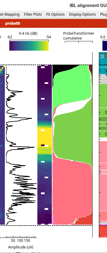
6. Choose XGBoost region prediction, and load it in the same way. It is a second model, trained on the same features. You will compare the two in step 6.

5. Predict the regions with the alignment model

The third model works differently. It predicts the features expected at every point along the histology track, and aligns the recorded features to them. Each channel then takes the atlas region of the point on the track where it was placed.

1. Choose Auto-alignment from the Prediction Plots menu, and click OK in the model’s dialog.

2. A progress dialog shows the alignment running. When it finishes, a result window opens.

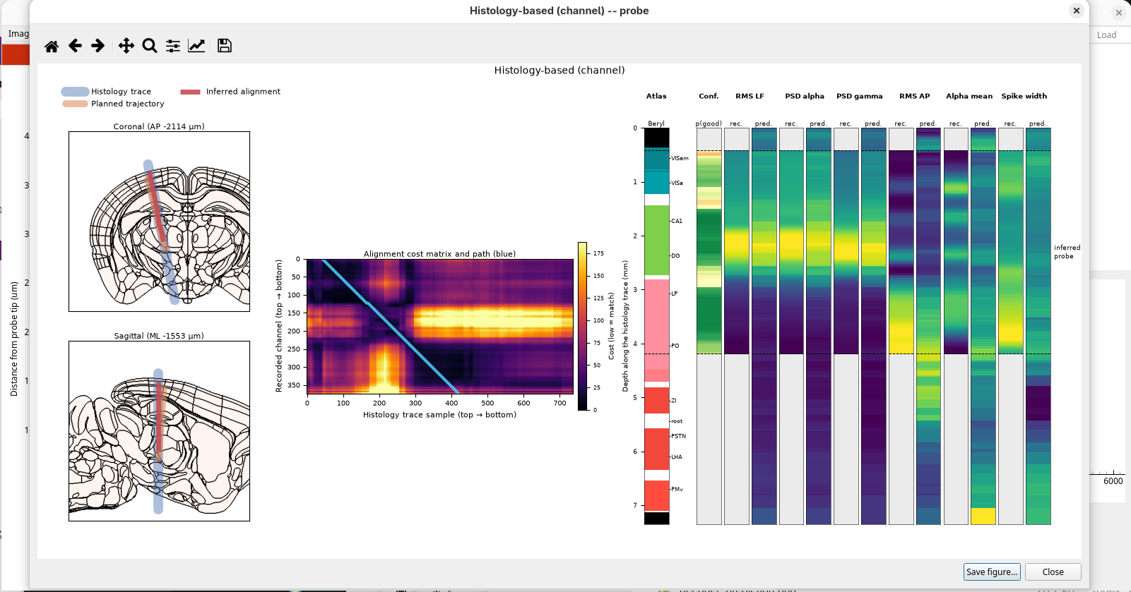
The result window shows how the model matched the recording to the track:

• the track on coronal and sagittal slices, with the alignment it found

• the cost matrix: every recorded channel against every point along the track, with the best path through it

• stripes along the track: the atlas regions, the confidence, and the recorded and predicted features

3. Close the result window. Back in the main window, the prediction panel shows the atlas region of each channel where the alignment model placed it on the track.

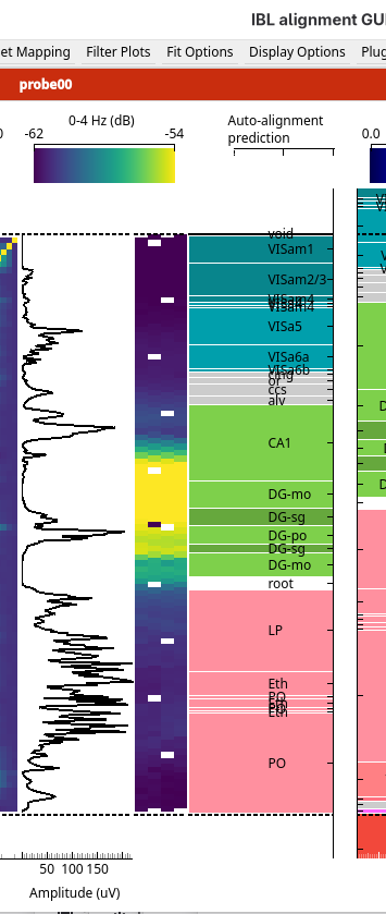
4. Choose Auto-alignment (confidence) to see how confident the alignment is along the probe: green is high, red is low.

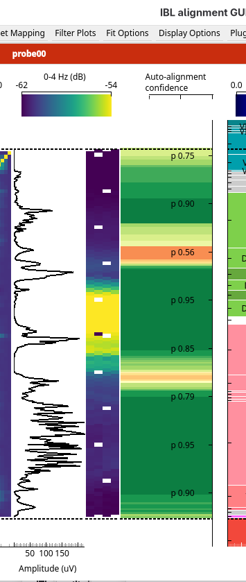
To see the result window again later, use Plugins → Channel Prediction → Show auto-alignment results.

6. Compare all the predictions

1. Press Shift+P. The ephys plots are replaced by every prediction side by side: the two region decoders, each with its cumulative probabilities, and the alignment model with its confidence.

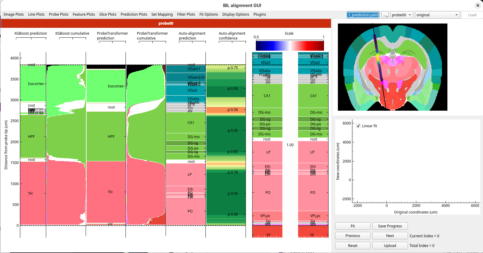
2. Compare the models. Boundaries that the models agree on, and that the alignment model is confident about, are the ones to trust most.

7. Use the predictions in your own alignment

The predictions do not change your alignment. They are a guide for placing reference lines, and you can place the lines in the all predictions view.

1. Add a reference line pair at each boundary the models agree on: the Ephys line on the predicted boundary, and the Histology line on the matching boundary in the Histology figure. Here they agree on three: the top of the brain, the boundary between the isocortex and the hippocampus, and the boundary between the hippocampus and the thalamus.

2. Press Enter to apply the fit.

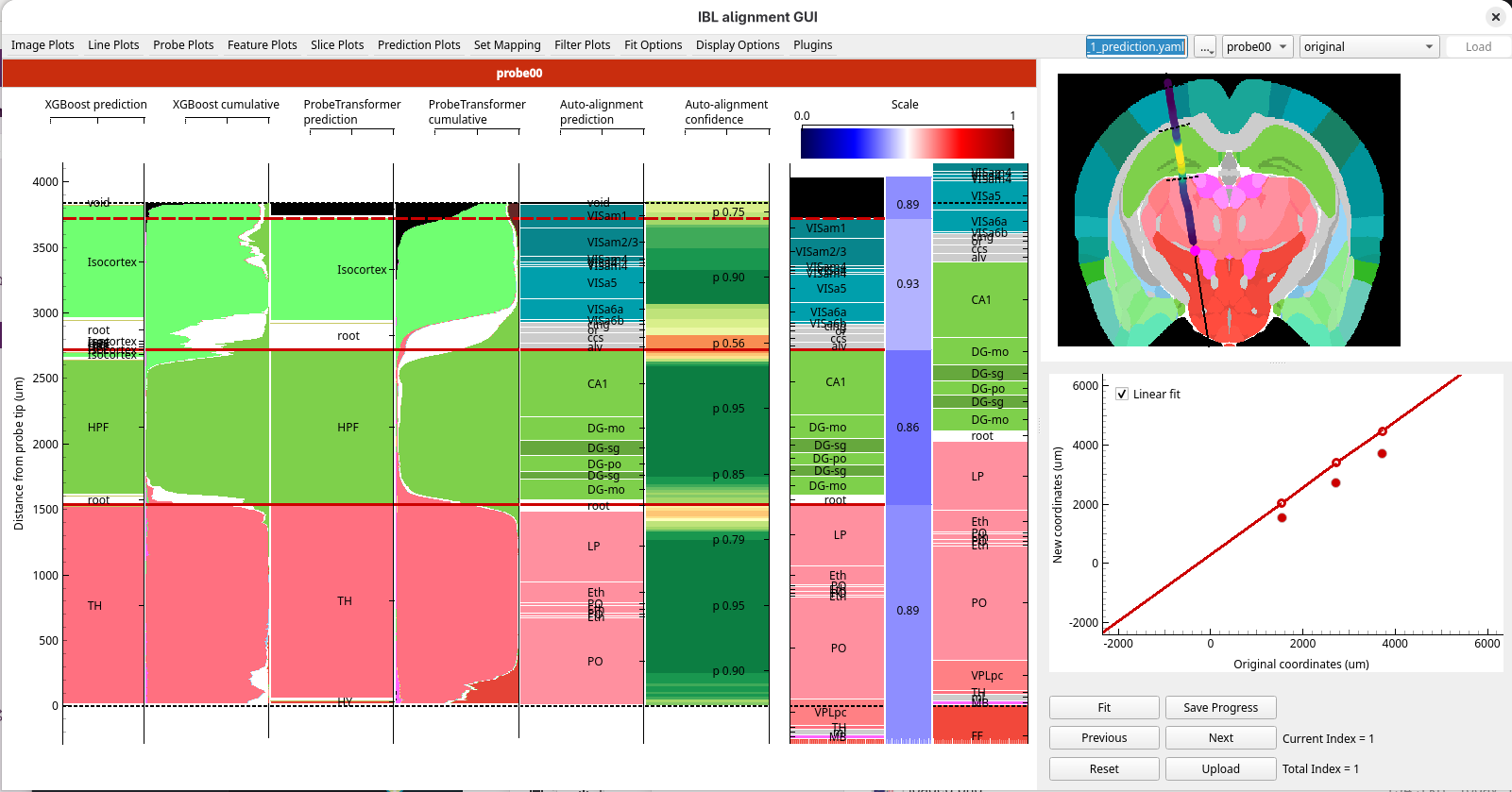
3. Choose any image plot to go back to the ephys plots, and check the alignment against the features you used in Your first alignment.

4. Upload with Shift+U when you are happy with it.

What you’ve learned

You have:

• loaded a session and its features from a session YAML

• predicted regions from the electrophysiology with three models, and compared them with the histology

• read the confidence of a prediction

• compared all the predictions side by side, and placed reference lines where they agree

Next steps

• The channel prediction models: what the models do, and their limits

• How to compute the features for a probe: compute features for your own recordings

• How to use a specific model release: use a different model release