Aligning a multi-shank probe with a second recording

In this tutorial you will align a four-shank Neuropixels probe, and learn two ways to get more out of your data when aligning.

The first is to look at all four shanks together. The shanks are fixed side by side on the probe and pass through similar anatomy, so a boundary on one shank should appear at a similar depth on its neighbours, and each shank’s alignment is a check on the others.

The second is to bring in another recording. In this session the channels of each shank only cover the bottom 700 µm, too short a stretch to show many boundaries. At the end of the experiment, a short recording was also made with a different channel map, spanning the whole length of each shank. You will load the two side by side and align them together, using the boundaries in the second recording to align the first.

Before you start

• Complete Your first alignment. This tutorial assumes you can add reference line pairs and apply a fit.

• Extract the Sample data 2 folder from the sample data. It holds two recordings of the same four-shank Neuropixels 2.0 (2.4) probe, in the same session, with 96 channels per shank:

  • dense: the main recording, with each shank’s channels packed together in its bottom 700 µm

  • sparse: a short recording of about 5 minutes, made at the end of the experiment, with each shank’s channels spread along almost 3 mm

  Each shank was spike sorted separately, so each one has its own entry in the session YAML: probe01a to probe01d.

1. Open the dense recording

The datasets of Sample data 2 are spread over several folders, so they are listed in a session YAML instead of being opened as one folder. Start with the YAML for the dense recording alone.

1. Open sample_data_2_dense.yaml, in the Sample data 2 folder, in a text editor.

2. Change the path on the first line to the folder you extracted Sample data 2 into:

   path: /path/to/ephys_alignment_sample_data/sample_data_2      # <- change this
   
   probes:
   
     probe01a:
       datasets:
         spike_sorting:
           path: dense/spike_sorting/probe01a
         raw_ephys:
           path: dense/raw_ephys/probe01a
         picks:
           path: picks/probe01a
         output:
           path: dense/alignment/probe01a
   
     probe01b:
       ...
   

   Every other path in the file is relative to this one and so can be left as is. The entries for probe01b, probe01c and probe01d follow the same pattern.

3. Save the file.

4. Start the GUI with the YAML:

   alignment-gui -y /path/to/ephys_alignment_sample_data/sample_data_2/sample_data_2_dense.yaml
   

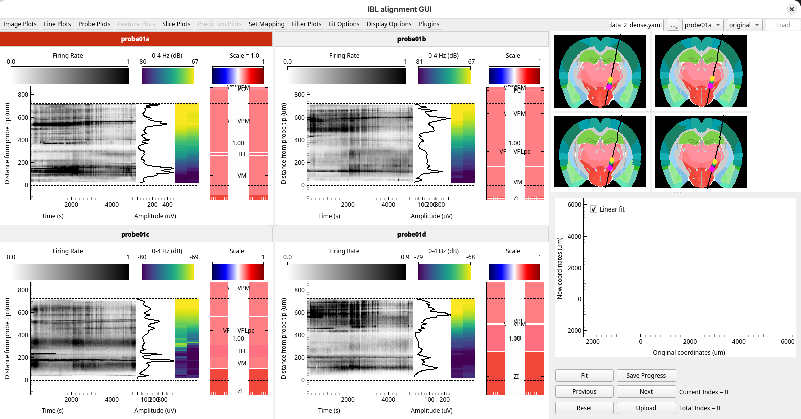
The data loads with the shanks side by side in a grid, each titled with its name. The title of the active shank is red.

2. Switch between the grid and the tabs

1. Press Right and Left to step through the shanks. The red title moves to show which shank is active.

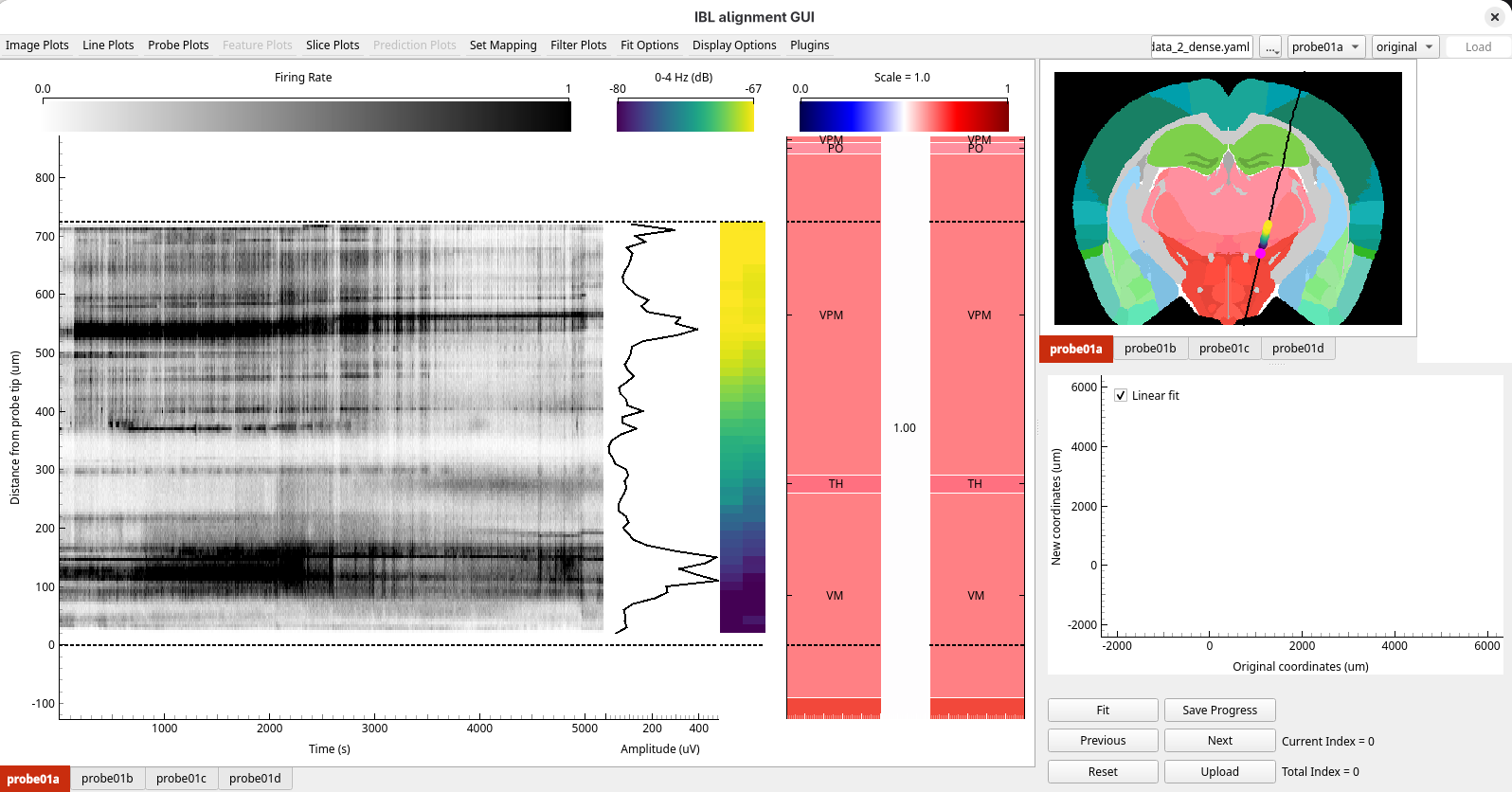
2. Press T. The layout changes to one tab per shank, and only the active shank is shown.

3. Press Right and Left again: each press moves to the next tab.

4. Press T to go back to the grid.

3. Look for landmarks

Cycle through the plots with Alt+1, Alt+2 and Alt+3, as in Your first alignment.

The channels of each shank span only 700 µm, so the probe passes through few regions on this stretch, and few features stand out. There are not enough clear boundaries to align to with confidence.

4. Bring in the second recording

At the end of the experiment, a short recording of about 5 minutes was also made with a different channel map, spanning the whole length of each shank. It is the same probe in the same tissue, so it can be aligned together with the dense recording. The GUI calls each recording a configuration.

The channel map of this recording is the SpikeGLX IMRO table NPtype2014_quarterDensity_ref1Tip0.imro, if you want to record with it yourself.

1. Open sample_data_2_dense_sparse.yaml in a text editor. It lists both recordings under configurations, each with its own probes:

   path: /path/to/ephys_alignment_sample_data/sample_data_2      # <- change this
   
   configurations:
   
     dense:
       probes:
   
         probe01a:
           datasets:
             spike_sorting:
               path: dense/spike_sorting/probe01a
             raw_ephys:
               path: dense/raw_ephys/probe01a
             picks:
               path: picks/probe01a
             output:
               path: dense/alignment/probe01a
   
         probe01b:
           ...
   
     sparse:
       probes:
   
         probe01a:
           datasets:
             spike_sorting:
               path: sparse/spike_sorting/probe01a
             processed_ephys:
               path: sparse/processed_ephys/probe01a
             picks:
               path: picks/probe01a
             output:
               path: sparse/alignment/probe01a
   
         probe01b:
           ...
   

   The dense configuration is the same as the YAML you opened before. Each shank has the same name, probe01a to probe01d, in both configurations: that is how the GUI knows they are the same shank. Both configurations use the same traced tracks, in picks, since the probe did not move. Each has its own output folder, so the results of one do not overwrite the other.

2. Change the path and save the file.

3. In the GUI, click ..., choose Open session YAML…, and choose sample_data_2_dense_sparse.yaml.

The data loads, and a configuration dropdown appears in the top right corner, after the alignment dropdown. It starts on the first configuration in the YAML, dense.

5. Look at the sparse recording

1. Open the configuration dropdown and choose sparse. The sparse recording is shown on its own, with the channels of each shank spread along almost 3 mm.

2. Select Firing Rate from the Image Plots menu. On every shank the firing stops at about 2000 µm: this probably indicates the boundary between the thalamus and the hippocampus.

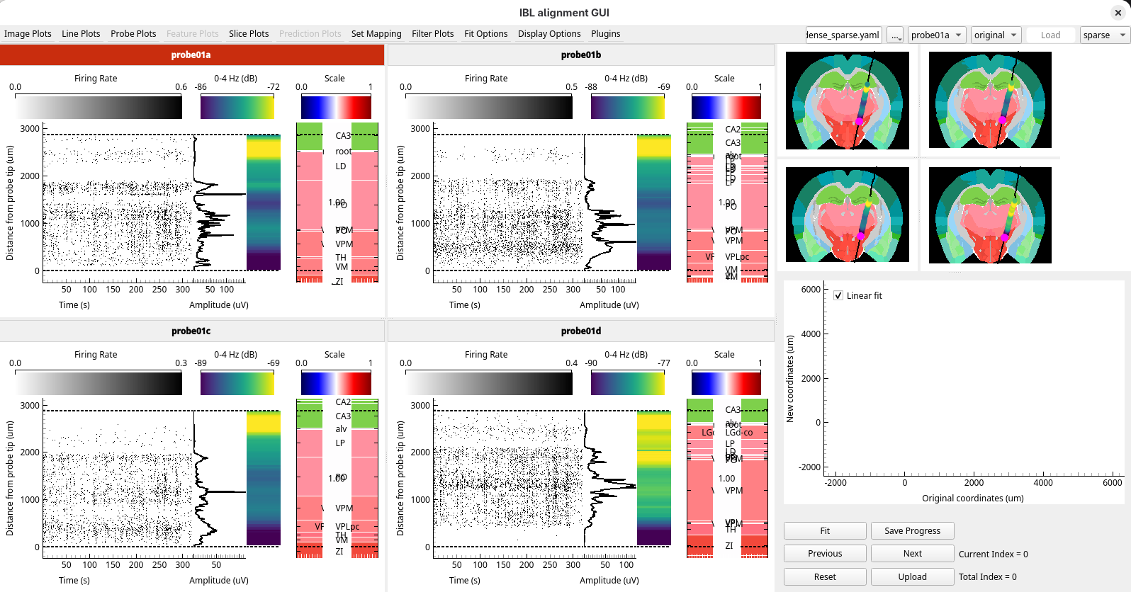
This boundary is well above the dense channels, which stop at 700 µm, so it could not be seen in the dense recording.

6. Show both configurations

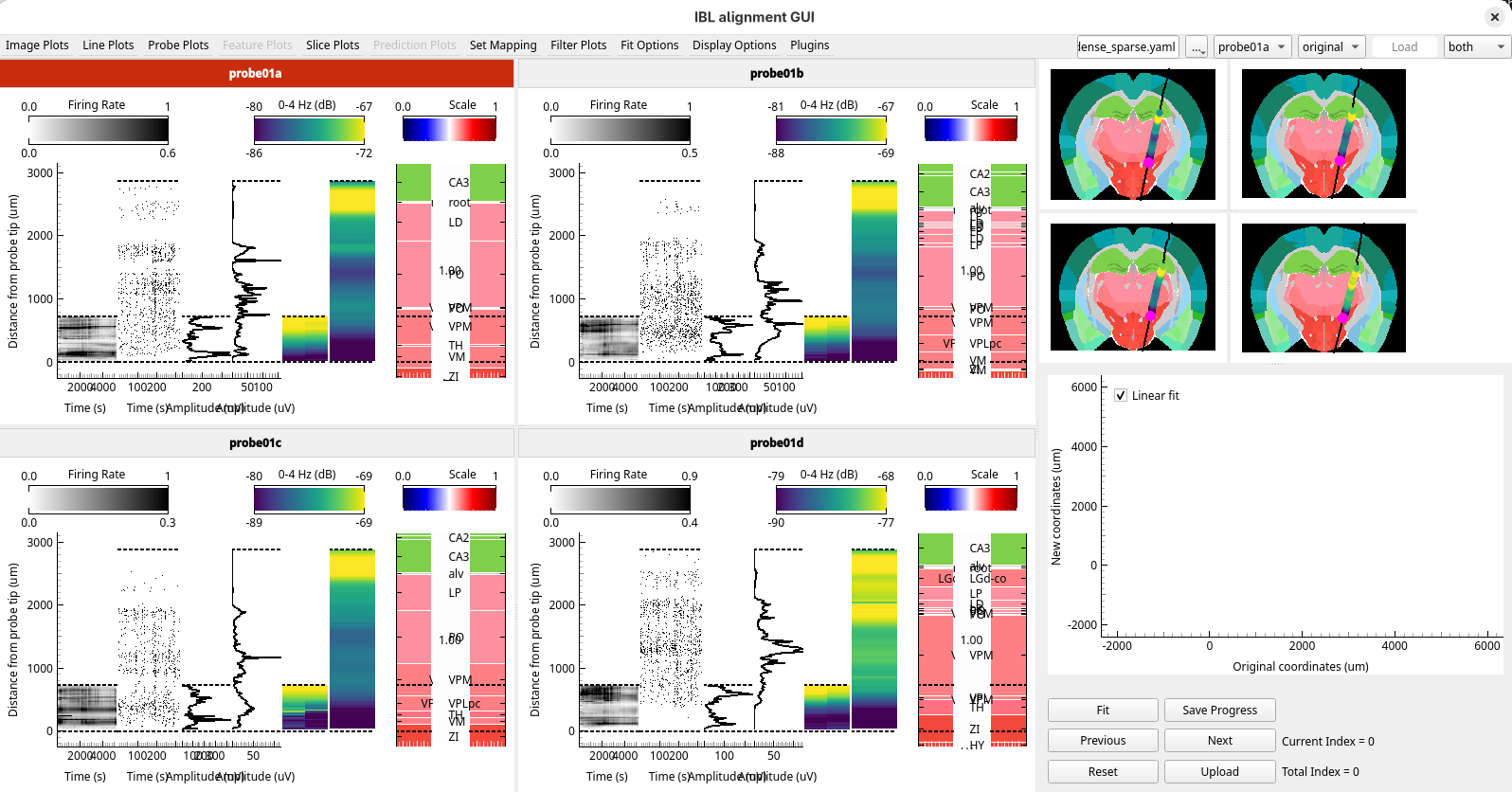
1. Choose both in the configuration dropdown. Each panel shows the two recordings next to each other: the dense one in the bottom 700 µm, and the sparse one along the whole shank.

7. Align using the sparse recording

1. Choose sparse in the configuration dropdown.

2. On probe01a, add a reference line pair: the Ephys line where the firing stops, at about 2000 µm, and the Histology line at the top of the thalamus, where the pink thalamic regions meet the green hippocampus.

3. Press Enter to apply the fit.

4. Do the same on probe01b, probe01c and probe01d. Press Right to move to the next shank, or double-click in its figures.

8. Compare the shanks

Look at the Fit figure. In the grid layout it shows the fit of every shank.

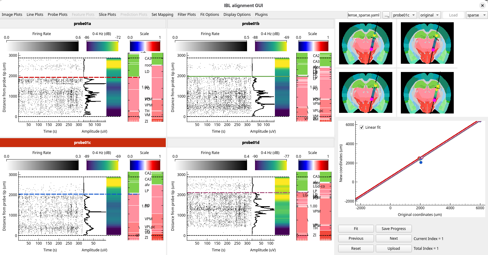
The fits of the four shanks should be offset by similar amounts. The shanks are fixed to the same base, so they are inserted together and cannot move along the track independently of each other. A shank whose fit is offset very differently from the others may be matched to a wrong boundary: check its reference lines against those of its neighbours.

9. See the alignment in both recordings

1. Choose both in the configuration dropdown.

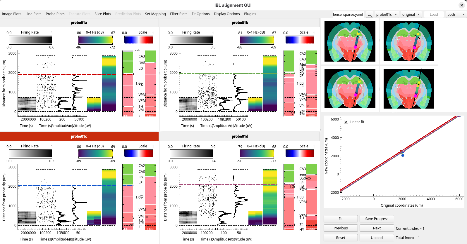
The reference lines you placed in the sparse recording are drawn in the dense one too: the two recordings come from the same probe, so they share one alignment. The fit stretches the histology of both, so the dense channels take their regions from the boundary you found in the sparse recording.

2. Choose dense. Its reference lines and fits are the ones you made in sparse.

10. Upload the alignment

1. Press Shift+U or click Upload. A dialog lists the shanks: tick all four and click OK.

2. Click Yes for each shank.

3. Open the Sample data 2 folder, and look in dense/alignment and sparse/alignment. Each has a folder per shank, and each of those has two new files:

   • prev_alignments.json, which holds the alignment. Open it for probe01a in both dense and sparse: the two are the same, because the recordings share one alignment.

   • channel_locations.json, which holds the position and brain region of every channel. It is different in dense and sparse, because the two channel maps put the channels in different places along the shank.

The alignment you made using the sparse recording now gives the brain region of every channel of the dense one.

What you’ve learned

You have:

• looked at the four shanks of a probe together, in the grid and tabbed layouts

• combined two recordings of the same probe, and switched between showing one and both

• aligned a recording with few landmarks using a boundary in a second recording

• used the fits of neighbouring shanks to check each other’s alignment

• uploaded one alignment for both recordings, and found the files for each

• written session YAMLs with one configuration and with two

Next steps

• Shanks, probes and configurations: how shanks, probes and configurations relate

• How to compare two versions of a recording: a session YAML with two configurations for your own data