How to access the IBL Brain-Wide Map LFP dataset

The IBL Brain-Wide Map (BWM) LFP dataset is distributed as a 16GB .h5 file containing 699 individual recordings of 384 channels each.

ImportantBefore you start

• Align with trial events via sr.times — each recording stores a sync-corrected session clock; always use sr.times rather than a manual np.arange / sr.fs when matching LFP samples to spike times or trial events. See Session-clock times.

• Use binned reads for brainwide sweeps — looping over all 699 recordings at full 384-channel resolution is memory-intensive. Pass bin_channels=4 to reduce each recording to 96 spatial bins with acceptable loss of depth coverage. See Binned-channel reads.

Visualise with viewephys

from lfpack import LFPackReader
from viewephys.gui import viewephys
from iblatlas.atlas import BrainRegions

file_lfpack = "lf_compressed_all_bwm.h5"
pid = 'dab512bd-a02d-4c1f-8dbc-9155a163efc0'

sr = LFPackReader(file_lfpack, recording=pid)
traces = sr[:5000, :].T         # (nc, n_samples)
eqc = viewephys(traces, fs=sr.fs, channels=sr.channels, br=br)   # viewephys expects (nc, n_samples)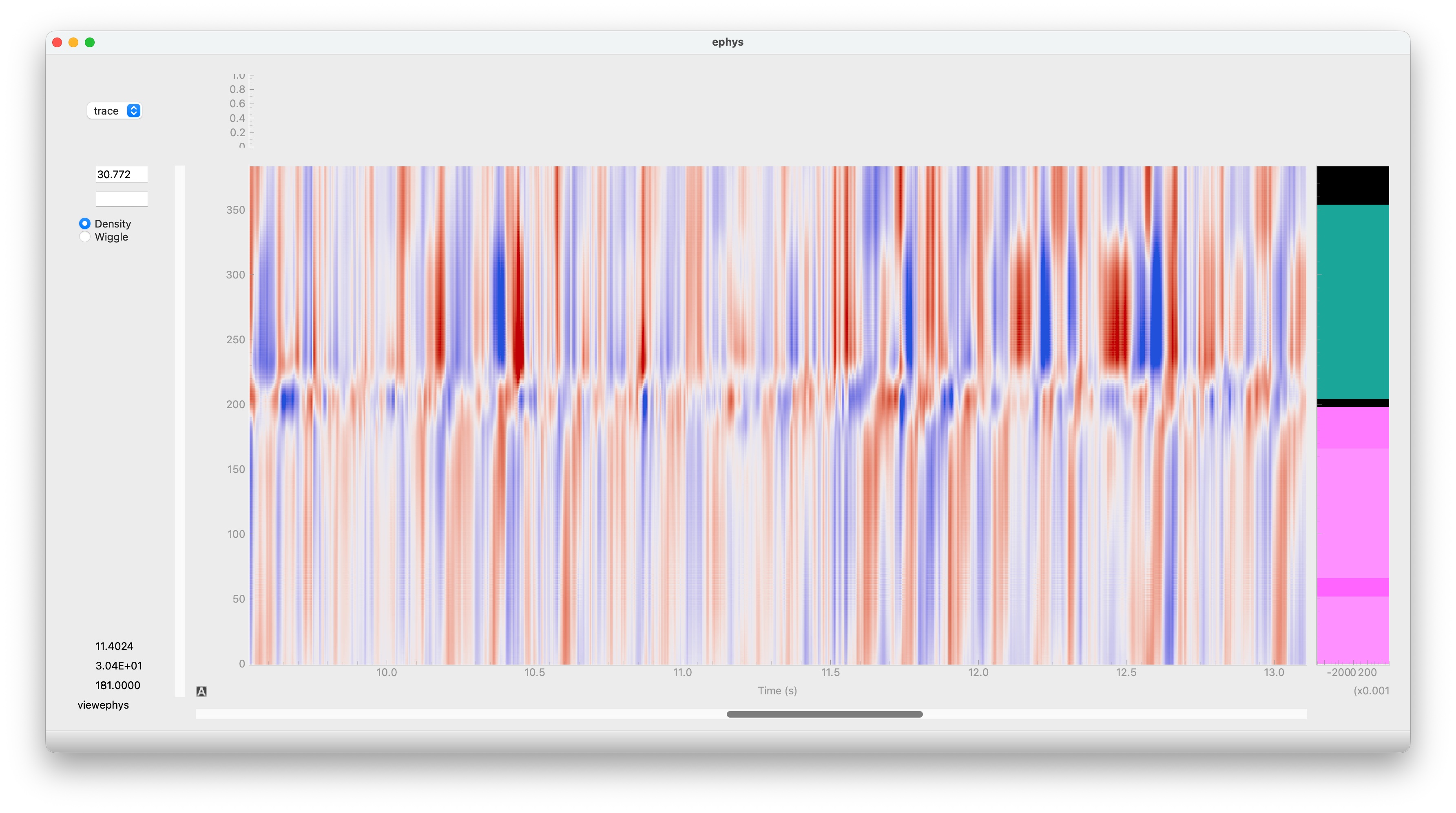

viewephys showing decompressed LFP for one BWM probe; the colour bar on the right indicates brain regions along the probe depth

Prerequisites

uv pip install lfpack viewephys one-api iblatlas

Download

From inside the ibl-ai-agent repository:

uv run python scripts/download_datasets.py --lfp

This downloads lf_compressed_all_bwm.h5 (~14 GB) into reports/datasets/bwm_lfp/ and writes the path into data_locations.local.yaml automatically.

Or, from Python (no AWS credentials needed — uses the ONE public S3 helper):

from one.remote.aws import s3_download_file

s3_download_file(
    source="resources/ibl-agent-data/lf_compressed_all_bwm.h5",
    destination="lf_compressed_all_bwm.h5",
)

s3_download_file defaults to the IBL public bucket, shows a tqdm progress bar, and skips the download if the local file already has the correct size.

List recordings

Each file contains one entry per BWM probe. Recording identifiers are named after the probe identifier UUID pid.

from lfpack import LFPackReader

recordings = LFPackReader.recordings("lf_compressed_all_bwm.h5")
print(f"{len(recordings)} recordings")
print(recordings[:3])
# 699 recordings
# ['00a824c0-e060-495f-9ebc-79c82fef4c67', '00a96dee-1e8b-44cc-9cc3-aca704d2b594', '00c425fd-ec3e-4cd2-b8af-c0bc0c4bdd44']

Read a single recording

from lfpack import LFPackReader

file_lfpack = "lf_compressed_all_bwm.h5"
pid = 'dab512bd-a02d-4c1f-8dbc-9155a163efc0'

sr = LFPackReader(file_lfpack, recording=pid)

# First 10 seconds — shape (2500, nc), float32, volts
traces = sr[: int(10 * sr.fs)].T

print(f"Duration:    {sr.ns / sr.fs:.1f} s")
print(f"Channels:    {sr.nc}")
print(f"Sample rate: {sr.fs} Hz")   # 250 Hz (decimated from 2500 Hz)
print(f"Shape:       {traces.shape}")

# Duration:    3668.9 s
# Channels:    384
# Sample rate: 250.00252518761928 Hz
# Shape:       (384, 2500)

LFPackReader is a drop-in for spikeglx.Reader. Slicing decompresses only the requested chunks — the full file is never loaded into memory.

Binned-channel reads

Adjacent channels are spatially correlated at LFP frequencies. Passing bin_channels sums neighbouring channels during decompression, reducing memory use. A factor of 4 takes 384 channels down to 96 while keeping depth resolution useful for LFP.

from lfpack import LFPackReader

file_lfpack = "lf_compressed_all_bwm.h5"
pid = 'dab512bd-a02d-4c1f-8dbc-9155a163efc0'

sr = LFPackReader(file_lfpack, recording=pid, bin_channels=4)

traces = sr[:, :]      # (ns, 96) — full recording, 96 spatial bins
print(sr.nc)           # 96
print(sr.geometry["y"])           # mean depth of each 4-channel group
print(sr.geometry_full['binned_channel_index'])  # spatial mapping of the original 384 channels into the 96 binned ones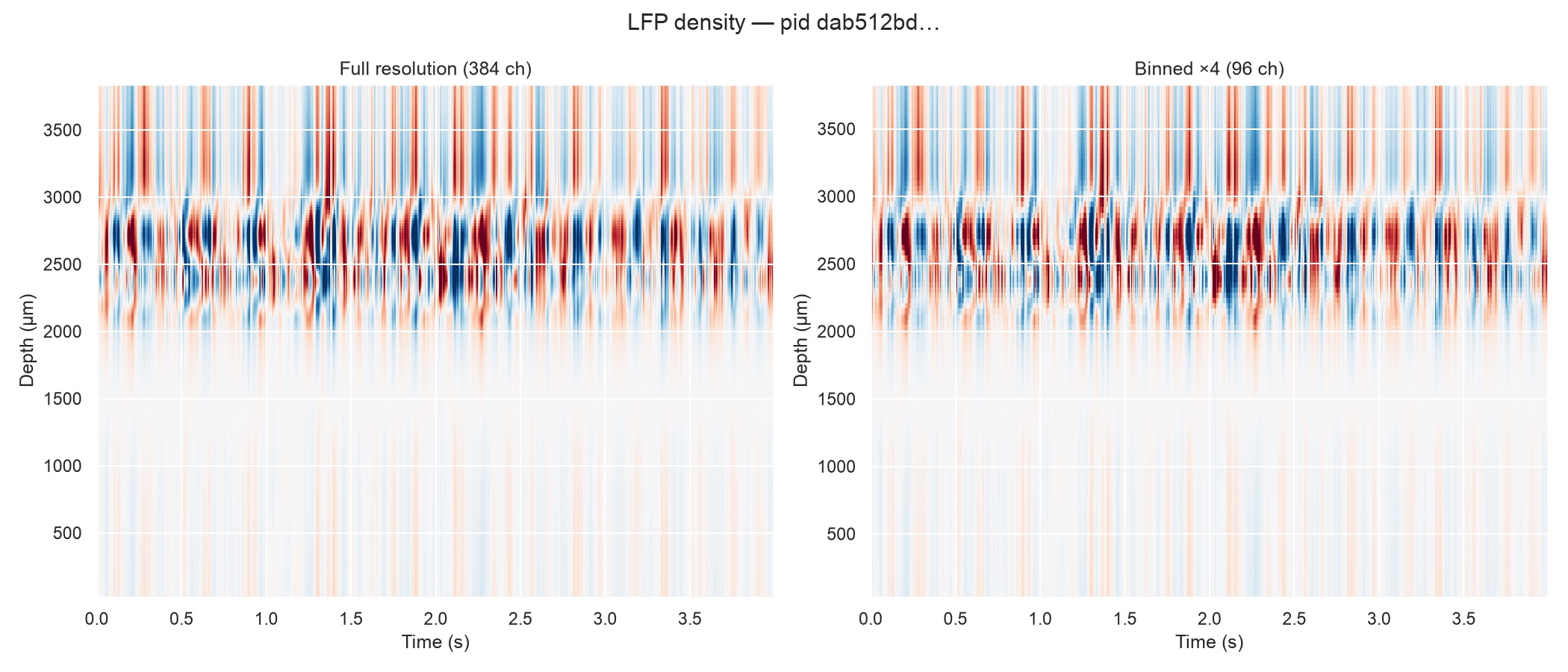

Full-resolution (384 ch) vs binned ×4 (96 ch) LFP density for the same 4-second window

Channel brain locations

Each recording stores per-channel brain location annotations embedded in the file — no network call needed. Access them via sr.channels:

from lfpack import LFPackReader

sr = LFPackReader("lf_compressed_all_bwm.h5", recording=pid)
ch = sr.channels

print(ch["acronym"][:5])   # ['VISp', 'VISp', 'CA1', 'CA1', 'DG']
print(ch["atlas_id"][:5])  # Allen CCF structure IDs, int32
print(ch["x"][:5])         # mediolateral MNI coordinates, metres
print(ch["y"][:5])         # anteroposterior
print(ch["z"][:5])         # dorsoventral

When using bin_channels, channels automatically aggregates: coordinates are averaged and brain region is the within-group mode:

sr = LFPackReader("lf_compressed_all_bwm.h5", recording=pid, bin_channels=4)
ch = sr.channels           # shapes (96,) — one entry per spatial bin
ch_full = sr.channels_full # shapes (384,) — always raw per-electrode

Session-clock times

sr.times returns a (ns,) array of session-clock timestamps (seconds) for every LFP sample, derived from the sync signal stored during compression. Use it to align LFP traces with trial events or spike times:

from lfpack import LFPackReader
import numpy as np

file_lfpack = "lf_compressed_all_bwm.h5"
pid = 'dab512bd-a02d-4c1f-8dbc-9155a163efc0'

sr = LFPackReader(file_lfpack, recording=pid)

n = int(10 * sr.fs)
traces = sr[:n, :]      # (n_samples, nc) — first 10 s
t = sr.times[:n]        # (n_samples,)    — session-clock seconds

# Align with trial events loaded via ONE
# stim_on = trials['stimOn_times']   # already in session-clock seconds
# idx = np.searchsorted(t, stim_on)  # nearest LFP sample for each stimulus onset