Atlas mapping

# import brain atlas and brain regions objects
from iblatlas.atlas import AllenAtlas
from iblatlas.regions import BrainRegions
ba = AllenAtlas()
br = BrainRegions() # br is also an attribute of ba so could to br = ba.regions

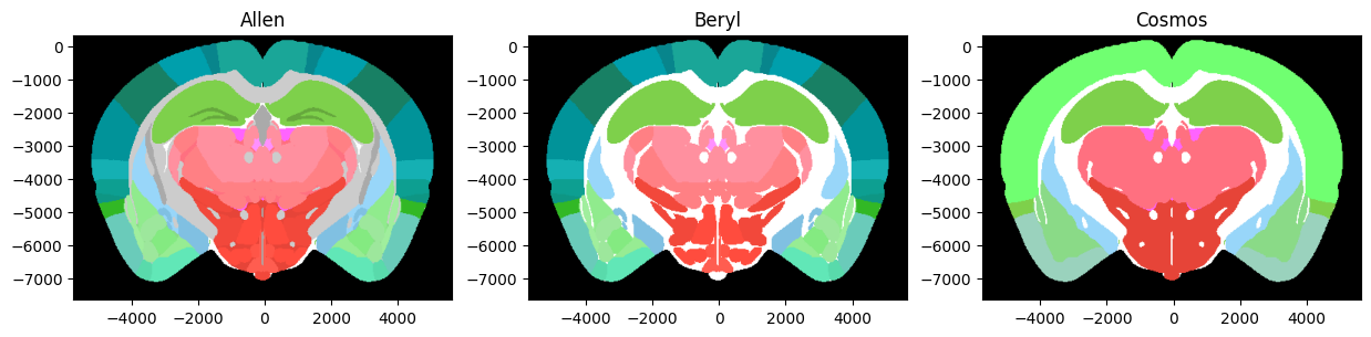
Available Mappings

Four mappings are currently available within the IBL, these are:

1. Allen Atlas - total of 1328 annotation regions provided by Allen Atlas

2. Beryl Atlas - total of 308 annotation regions

3. Cosmos Atlas - total of 12 annotation regions

4. Swanson Atlas - total of 319 annotation regions (*)

(*) Note: The dedicated mapping for plotting on Swanson flatmap is explained in this webpage.

# create figure
import matplotlib.pyplot as plt
fig, axs = plt.subplots(1, 3, figsize=(15, 18))

# plot coronal slice at ap = -2000 um
ap = -2000 / 1e6
# Allen mapping
ba.plot_cslice(ap, volume='annotation', mapping='Allen', ax=axs[0])
_ = axs[0].set_title('Allen')
# Beryl mapping
ba.plot_cslice(ap, volume='annotation', mapping='Beryl', ax=axs[1])
_ = axs[1].set_title('Beryl')
# Cosmos mapping
ba.plot_cslice(ap, volume='annotation', mapping='Cosmos', ax=axs[2])
_ = axs[2].set_title('Cosmos')

The br.mappings contains the index of the region for a given mapping. You can use these indices to find for example the acronyms contained in Cosmos:

import numpy as np
cosmos_indices = np.unique(br.mappings['Cosmos'])
br.acronym[cosmos_indices]

array(['void', 'root', 'Isocortex', 'OLF', 'HPF', 'CTXsp', 'CNU', 'TH',
       'HY', 'MB', 'HB', 'CB'], dtype=object)

You can check that all brain regions within these 4 mappings are contained in the Allen parcellation, for example for Beryl:

set(np.unique(br.mappings['Beryl'])).difference(set(np.unique(br.mappings['Allen'])))
# Expect to return an empty set

set()

Understanding the mappings

The mappings store the highest level annotation (or parent node) that should be considered. Any regions that are children of these nodes are assigned the same annotation as their parent.

For example, consider the region with the acronym MDm (Mediodorsal nucleus of the thalamus, medial part). Firstly, to navigate ourselves, we can find the acronyms of all the ancestors to this region,

# First find the atlas_id associated with acronym MDm
atlas_id = br.acronym2id('MDm')
# Then find the acronyms of the ancestors of this region
print(br.ancestors(ids=atlas_id)['acronym'])

['root' 'grey' 'BS' 'IB' 'TH' 'DORpm' 'MED' 'MD' 'MDm']

We can then take a look at what acronym this region will be assigned under the different mappings. Under the Allen mapping we expect it to be assigned the same acronym as this is the lowest level region parcelation that we use.

print(br.acronym2acronym('MDm', mapping='Allen'))

['MDm']

Under the Beryl mapping, MDm is given the acronym of it’s parent, MD

print(br.acronym2acronym('MDm', mapping='Beryl'))

['MD']

Under the Cosmos mapping, it is assigned to the region TH

print(br.acronym2acronym('MDm', mapping='Cosmos'))

['TH']

Under the Swanson mapping, it is assigned to the region MD

print(br.acronym2acronym('MDm', mapping='Swanson'))

['MD']

Therefore any clusters that are assigned an acronym MDm in the Allen mapping, will instead be assigned to the region MD in the Beryl or Swanson mapping, and TH in the Cosmos mapping.

If a region is above (i.e. parent) of what is included in a mapping, the value for this region is set to root. For example TH is not included in the Beryl nor Swanson mapping

print(br.acronym2acronym('TH', mapping='Beryl'))

['root']

print(br.acronym2acronym('TH', mapping='Swanson'))

['root']

However, a child region that is not included in the mapping will be returned as its closest parent in the mapping. For example, VISa is not included in Swanson, but its parent PLTp is:

print(br.acronym2acronym('VISa', mapping='Swanson'))

['VISa']

Lateralisation

Lateralised versions of each of the three mappings are also available. This allow regions on the left and right hemispheres of the brain to be differentiated.

The convention used is that regions in the left hemisphere have negative atlas ids whereas those on the right hemisphere have positive atlas ids.

For the non lateralised mappings the atlas id is always positive regardless of whether the region lies in the left or right hemisphere. Aggregating values over regions could result, therefore, in values from different hemispheres being considered together.

One thing to be aware of, is that while lateralised mappings return distinct atlas ids for the left and right hemispheres, the acronyms returned are not lateralised.

For example consider finding the atlas id when mapping the acronym MDm onto the Beryl atlas. When specifying the left hemisphere, the returned atlas id is negative

# Left hemisphere gives negative atlas id
print(br.acronym2id('MDm', mapping='Beryl-lr', hemisphere='left'))

[-362]

When specifying the right hemisphere, the returned atlas id is positive

# Left hemisphere gives negative atlas id
print(br.acronym2id('MDm', mapping='Beryl-lr', hemisphere='right'))

[362]

However, when converting from atlas id to acronym, regardless of whether we specify a negative (left hemisphere) or positive (right hemisphere) value, the returned acronym is always the same

print(br.id2acronym(-362, mapping='Beryl-lr'))

['MD']

print(br.id2acronym(362, mapping='Beryl-lr'))

['MD']

How to map your data

Mapping from mlapdv coordinates

The recommended and most versatile way to find the locations of clusters under different mappings is to use the mlapdv coordinates of the clusters. Given a probe insertion id, the clusters object can be loaded in using the following code

from brainbox.io.one import SpikeSortingLoader
from one.api import ONE
one = ONE()

pid = 'da8dfec1-d265-44e8-84ce-6ae9c109b8bd'

sl = SpikeSortingLoader(pid=pid, one=one, atlas=ba)
spikes, clusters, channels = sl.load_spike_sorting()
clusters = sl.merge_clusters(spikes, clusters, channels)

/opt/hostedtoolcache/Python/3.12.7/x64/lib/python3.12/site-packages/one/alf/files.py:10: FutureWarning: `one.alf.files` will be removed in version 3.0. Use `one.alf.path` instead.
  warnings.warn(
/opt/hostedtoolcache/Python/3.12.7/x64/lib/python3.12/site-packages/one/util.py:543: ALFWarning: Multiple revisions: "", "2024-05-06"
  warnings.warn(f'Multiple revisions: {rev_list}', alferr.ALFWarning)
/opt/hostedtoolcache/Python/3.12.7/x64/lib/python3.12/site-packages/one/util.py:543: ALFWarning: Multiple revisions: "", "2024-05-06"
  warnings.warn(f'Multiple revisions: {rev_list}', alferr.ALFWarning)

You will find that the cluster object returned already contains an atlas_id attribute. These are the atlas ids that are obtained using the default mapping - non lateralised Allen. For this mapping regardless of whether the clusters lie in the right or left hemisphere the clusters are assigned positive atlas ids

print(clusters['atlas_id'][0:10])

[596 596 596 596 596 596 596 596 596 596]

We can obtain the mlapdv coordinates of the clusters and explore in which hemisphere the clusters lie, clusters with negative x lie on the left hemisphere.

import numpy as np
mlapdv = np.c_[clusters['x'], clusters['y'], clusters['z']] # x = ml, y = ap, z = dv
clus_LH = np.sum(mlapdv[:, 0] < 0)
clus_RH = np.sum(mlapdv[:, 0] > 0)
print(f'Total clusters = {len(mlapdv)}, LH clusters = {clus_LH}, RH clusters = {clus_RH}')

Total clusters = 914, LH clusters = 914, RH clusters = 0

To get a better understanding of the difference between using lateralised and non-lateralised mappings, let’s also make a manipulated version of the mlapdv positions where the first 5 clusters have been moved into the right hemisphere and call this mlapdv_rh

mlapdv_rh = np.copy(mlapdv)
mlapdv_rh[0:5, 0] = -1 * mlapdv_rh[0:5, 0]
clus_LH = np.sum(mlapdv_rh[:, 0] < 0)
clus_RH = np.sum(mlapdv_rh[:, 0] > 0)
print(f'Total clusters = {len(mlapdv_rh)}, LH clusters = {clus_LH}, RH clusters = {clus_RH}')

Total clusters = 914, LH clusters = 909, RH clusters = 5

To find the locations of the clusters in the brain from the mlapdv position we can use the get_labels method in the AllenAtlas object. First let’s explore the output of using a non lateralised mapping.

atlas_id_Allen = ba.get_labels(mlapdv, mapping='Allen')
atlas_id_Allen_rh = ba.get_labels(mlapdv_rh, mapping='Allen')
print(f'Non-lateralised Allen mapping ids using mlapdv: {atlas_id_Allen[0:10]}')
print(f'Non-lateralised Allen mapping ids using mlapdv_rh: {atlas_id_Allen_rh[0:10]}')

Non-lateralised Allen mapping ids using mlapdv: [596 596 596 596 596 596 596 596 596 596]
Non-lateralised Allen mapping ids using mlapdv_rh: [596 596 596 596 596 596 596 596 596 596]

Notice that regardless of whether the clusters lie in the left or right hemisphere the sign of the atlas id is the same. The result of this mapping is also equivalent the default output from clusters['atlas_id']

np.array_equal(clusters['atlas_id'], atlas_id_Allen)

True

Now if we use the lateralised mapping, we notice that the clusters in the left hemisphere have been assigned negative atlas ids whereas those in the right hemisphere have positive atlas ids

atlas_id_Allen = ba.get_labels(mlapdv, mapping='Allen-lr')
atlas_id_Allen_rh = ba.get_labels(mlapdv_rh, mapping='Allen-lr')
print(f'Lateralised Allen mapping ids using mlapdv: {atlas_id_Allen[0:10]}')
print(f'Lateralised Allen mapping ids using mlapdv_rh: {atlas_id_Allen_rh[0:10]}')

Lateralised Allen mapping ids using mlapdv: [-596 -596 -596 -596 -596 -596 -596 -596 -596 -596]
Lateralised Allen mapping ids using mlapdv_rh: [ 596  596  596  596  596 -596 -596 -596 -596 -596]

By changing the mapping argument that we pass in, we can also easily obtain the atlas ids for the Beryl and Cosmos mappings

atlas_id_Beryl = ba.get_labels(mlapdv_rh, mapping='Beryl-lr')
atlas_id_Cosmos = ba.get_labels(mlapdv_rh, mapping='Cosmos')
print(f'Lateralised Beryl mapping ids using mlapdv_rh: {atlas_id_Beryl[0:10]}')
print(f'Non-lateralised Cosmos mapping ids using mlapdv_rh: {atlas_id_Cosmos[0:10]}')

Lateralised Beryl mapping ids using mlapdv_rh: [ 596  596  596  596  596 -596 -596 -596 -596 -596]
Non-lateralised Cosmos mapping ids using mlapdv_rh: [623 623 623 623 623 623 623 623 623 623]

Mapping from atlas ids

Methods are available that allow you to translate atlas ids from one mapping to another.

# map atlas ids from lateralised Allen to lateralised Beryl
atlas_id_Allen = ba.get_labels(mlapdv_rh, mapping='Allen-lr') # lateralised Allen

remap_beryl = br.id2id(atlas_id_Allen, mapping='Beryl-lr')
print(f'Lateralised Beryl mapping ids using remap: {remap_beryl[0:10]}')

# map atlas ids from lateralised Allen to non-lateralised Cosmos
remap_cosmos = br.id2id(atlas_id_Allen_rh, mapping='Cosmos')
print(f'Non-lateralised Cosmos mapping ids using remap: {remap_cosmos[0:10]}')

Lateralised Beryl mapping ids using remap: [ 596  596  596  596  596 -596 -596 -596 -596 -596]
Non-lateralised Cosmos mapping ids using remap: [623 623 623 623 623 623 623 623 623 623]

When remapping with atlas ids it is not possible to map from

1. A non-lateralised to a lateralised mapping.

2. From a higher mapping to a lower one (e.g cannot map from Beryl to Allen, or Cosmos to Allen)

3. From Beryl to Cosmos

This is why it is recommened to use mlapdv coordinates for remappings as it allows complete flexibility

Converting to acronyms

Methods are available to convert between atlas ids and acronyms. Note that when converting to acronyms, even if the atlas ids are lateralised the returned acronyms are not

atlas_id_Allen = ba.get_labels(mlapdv_rh, mapping='Allen-lr') # lateralised Allen
acronym_Allen = br.id2acronym(atlas_id_Allen, mapping='Allen-lr')
print(f'Acronyms of lateralised Allen ids: {acronym_Allen[0:10]}')

atlas_id_Allen = ba.get_labels(mlapdv_rh, mapping='Allen-lr') # Non-ateralised Allen
acronym_Allen = br.id2acronym(atlas_id_Allen)
print(f'Acronyms of non-lateralised Allen: {acronym_Allen[0:10]}')

Acronyms of lateralised Allen ids: ['NDB' 'NDB' 'NDB' 'NDB' 'NDB' 'NDB' 'NDB' 'NDB' 'NDB' 'NDB']
Acronyms of non-lateralised Allen: ['NDB' 'NDB' 'NDB' 'NDB' 'NDB' 'NDB' 'NDB' 'NDB' 'NDB' 'NDB']

It is also possible to simultaneously remap the acronyms with these methods

acronym_Cosmos = br.id2acronym(atlas_id_Allen, mapping='Cosmos-lr')
print(acronym_Cosmos[0:10])

['CNU' 'CNU' 'CNU' 'CNU' 'CNU' 'CNU' 'CNU' 'CNU' 'CNU' 'CNU']