Getting Started

This guide will walk you through the basic usage of the IBL Alignment GUI.

1. Sample Data

We provide a sample dataset to help you quickly get started with the tool. Download the sample data here.

Extract the contents to a location on your computer - you’ll need this path when loading data into the GUI.

• Sample data 1 contains data from a single shank NP3B probe insertion with 384 channels.

• Sample data 2 contains data from a four shank NP2.4 probe with 96 channels per shank.

2. Launching the GUI

After installation, launch the alignment GUI (with your virtual environment activated):

alignment-gui

A window containing blank plots should appear.

3. Loading Data

Once the GUI has launched, you’ll see a button in the top right corner with the symbol ...

Click this button and navigate to the folder containing your extracted sample data and load in Sample data 1.

After selecting the folder, click Load to load the data into the GUI.

4. Overview of Layout

The GUI consists of four main figures, each displaying a different aspect of the alignment process.

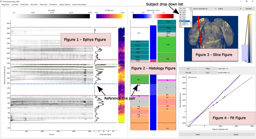
Figure 1: Ephys Figure

The Ephys figure contains three panels that display electrophysiology-related data in different formats:

Image Plots

2D representation of data displayed in images or scatter plots

Line Plots

1D representation of data displayed in a line plot

Probe Plots

2D representations of data overlaid on the probe geometry

You can switch between plots using either the Image Plots, Line Plots, and Probe Plots menu bars or the following keyboard shortcuts:

Shortcut	Action
Alt+1 / Shift+Alt+1	Image plots (forward / backward)
Alt+2 / Shift+Alt+2	Line plots (forward / backward)
Alt+3 / Shift+Alt+3	Probe plots (forward / backward)

Filtering Units

By default, the Ephys plots display all units classified as Good and MUA during spike sorting.

To restrict which units are shown, use the Filter Plots option in the menu bar. This allows you to selectively display specific unit classes, making it easier to focus on well-isolated units during alignment.

Figure 2: Histology Figure

The Histology figure displays the brain regions through which the traced probe track passes (the trajectory). It is divided into three panels, shown from left to right:

Scaled brain regions (left)

Brain regions after scaling has been applied based on reference lines

Scale factor heatmap (middle)

Heatmap showing the scaling applied to each region along the trajectory

Original brain regions (right)

Unscaled reference brain regions

Black dotted lines in the left and right panels indicate the positions of the most ventral and most dorsal electrodes along the trajectory.

Brain region labels overlaid on the histology can be toggled on and off:

Shortcut	Action
Shift+L	Toggle brain region labels

When hovering over a region in the central (scale factor) panel, the scale factor is displayed in the title of the colour bar at the top of the figure.

Figure 3: Slice Figure

The Slice figure displays a slice through the brain at the location of the traced probe trajectory.

Each slice layer is derived from the trajectory coordinate at that depth. As a result, if the trajectory is not smooth, the image may appear to jump between slices in some regions.

Overlaid on the slice are:

• A black line connecting the traced trajectory points and extended to the top and bottom of the brain

• Points indicating the locations of electrodes along the trajectory, coloured by the current feature displayed in the probe plots of the Ephys figure

When reference lines are added in the Ephys and Histology figures, they are displayed as black dotted lines perpendicular to the local trajectory.

The overlaid lines and electrode markers can be toggled on and off:

Shortcut	Action
Shift+C	Toggle trajectory overlay and electrode markers

The intensity of the slice image can be adjusted using the intensity scale bar on the right-hand side of the figure.

Slice Display Options

There are four available slice types, selectable via the Slice Plots menu bar or the following shortcuts:

Shortcut	Action
Alt+3 / Shift+Alt+3	Cycle through slice types (forward / backward)

The options are:

• Red channel of the histology image

• Green channel of the histology image

• Allen Brain Atlas average template

• Allen Brain Atlas annotation template

Note

The red and green histology channels are optional inputs and will not be displayed if not provided.

Figure 4: Fit Figure

The Fit figure provides a 2D visualization of the scaling applied along the depth of the probe trajectory.

Two lines are displayed:

Fit line

Shows the piecewise fit applied along the depth of the trajectory. The points indicate the positions of reference lines.

Linear fit line (dotted)

Displays a linear fit through all reference lines (only appears when 3+ reference lines are used)

Rescaling and Zoom

You can zoom into plots in the Ephys, Histology and Slice figures for closer inspection.

To reset the axes to their default limits:

Shortcut	Action
Shift+A	Reset axes to default limits

5. Alignment Workflow

Alignment between electrophysiology and histology data is achieved using reference line pairs.

Adding Reference Lines

A reference line pair can be added by double-clicking anywhere in either the Ephys or Histology figure.

This creates a pair of lines with matching colour and style, one in each figure. Each line can be moved independently.

Once both lines are positioned on corresponding features or landmarks, apply the fit:

Shortcut	Action
Click Fit button	Apply fit
Enter / Shift+Right	Apply fit

Fit Behaviour

The type of fit applied depends on the number of reference line pairs:

One reference line pair

Applies a simple offset along the trajectory

Two reference line pairs

Applies an offset and scaling between the two reference lines. Regions outside the reference lines are offset but remain unscaled.

Three or more reference line pairs

Applies an offset and piecewise scaling between each adjacent pair. By default, regions beyond the reference lines are scaled according to a global linear fit.

To prevent scaling outside the reference lines, disable the default behaviour by unchecking the Linear Fit checkbox in the top-left corner of the Fit figure.

When a fit is applied, the electrode locations shown in the Slice figure update automatically.

Previous Fits

Up to 10 previous fits are stored in memory.

You can navigate through previous fits:

Shortcut	Action
Click Previous / Next buttons	Navigate through fit history
Shift+Left / Shift+Right	Navigate through fit history

This allows you to quickly compare different alignment solutions.

Resetting the Fit

To reset the GUI to its original state (i.e. with no alignments applied):

Shortcut	Action
Click Reset button	Reset all alignments
Shift+R	Reset all alignments

Managing Reference Lines

Shortcut	Action
Shift+D	Delete reference line (hover over line first)
Shift+H	Hide / show all reference lines

Warning

Deleting a reference line also removes any fits that depend on it.

6. Saving Alignment Results

Once you are satisfied with the alignment, save the updated electrode locations:

Shortcut	Action
Click Upload button	Save alignment results
Shift+U	Save alignment results

This saves the following files in the output data directory:

channel_locations.json

Contains the updated electrode locations

prev_alignments.json

Stores the reference lines used for alignment, allowing previous alignments to be reloaded later

You will notice in the dropdown menu next to the Load button in the top left corner of the GUI that this new alignment is now available to load.

7. Loading Multi-Shank Data

Sample Data 2 contains recordings from a four-shank NP2.4 probe, and can be used to demonstrate the multi-shank capabilities of the GUI.

To load the data:

1. Click the ... button in the top-right corner of the GUI.

2. Navigate to the directory containing Sample Data 2.

3. Select the folder and click Load.

Once loaded, four panels will appear in the GUI window, one for each shank.

Working with Multiple Shanks

The alignment workflow is identical to that described for single-shank data. However, you can now switch between shanks:

Shortcut	Action
Click shank tabs	Switch between shanks
Left / Right	Switch between shanks

Although alignment is performed independently for each shank, the GUI allows all shanks to be visualised simultaneously. This is particularly useful for ensuring consistency across shanks and for accounting for mechanical constraints of the probe during alignment.

Tabbed and Non-Tabbed Views

Two display modes are available when working with multi-shank data:

• Tabbed view: Each shank displayed under its own tab

• Non-tabbed view: All shanks displayed simultaneously

You can toggle between these modes:

Shortcut	Action
Click Tabbed View in Display menu	Toggle view mode
Shift+T	Toggle view mode

In the non-tabbed view:

• The Fit figure shows fit lines for all shanks simultaneously

• The currently active shank is highlighted in red in the title bar of each figure

You can change the active shank using Left / Right arrow keys, or by clicking directly on the tabs.

Uploading Alignments

After pressing the Upload button, a dialog will appear asking whether to upload alignments for all shanks or only the active shank.

The data will be saved in the same way as for single-shank data, with each shank’s results saved in separate files with appropriate suffixes (e.g., channel_locations_shank_1.json).

Resources

An introduction to the tool was given at the 2020 UCL Neuropixels course. The lecture can be found here.