Download tutorial notebook Github link

Exploring the public IBL data with ONE

This tutorial will give an introduction into the publicly available data and show how to download electrophysiology data for a probe insertion and display a simple raster plot

First let’s get started by importing the ONE module and connecting to the database

# Import one and connect to the database
from one.api import ONE
one = ONE(base_url='https://openalyx.internationalbrainlab.org', silent=True)

We want to see what probe insertions are available on the database. To list them we can use the following command

eid = one.search()[0]
probe_insertions = one.load_dataset(eid, 'probes.description')

We can find the number of probes insertions available and some information about the first probe

from pprint import pprint
print(f'N probes = {len(probe_insertions)}')
pprint(probe_insertions[0])

N probes = 2
{'label': 'probe00',
 'model': '3B2',
 'raw_file_name': 'D:/iblrig_data/Subjects/SWC_043/2020-09-21/001/raw_ephys_data/_spikeglx_ephysData_g0/_spikeglx_ephysData_g0_imec0/_spikeglx_ephysData_g0_t0.imec0.ap.bin',
 'serial': 19108320031}

Datasets associated with each probe insertion are contained within a collection named ‘alf/’, where is the probe insertion label.

probe = probe_insertions[0]['label']

datasets = one.list_datasets(eid, collection=f'*/{probe}')
print(f'N datasets = {len(datasets)}')
pprint(datasets[0])

N datasets = 44
'alf/probe00/_kilosort_whitening.matrix.npy'

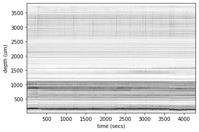
We are interested in downloading the spikes datasets output from spike sorting in order to display a raster plot of the neural activity recorded on the probe. To download the data we can use the following approach

spikes = one.load_object(eid, 'spikes',
                         collection=f'alf/{probe}', attribute=['times', 'depths', 'amps'])

We can import a module from brainbox that plots the raster across time

Note.

Requires ibllib to be installed.

from brainbox.plot import driftmap
driftmap(spikes['times'], spikes['depths'], t_bin=0.1, d_bin=5);