ONE Introductory Tutorial
In this tutorial we will use ONE to load IBL behavioural data and perform some simple analysis to assess the performance of a chosen subject during the IBL task.
Let’s get started by importing the ONE module and setting up a connection,
[1]:
from one.api import ONE
one = ONE(base_url='https://alyx.internationalbrainlab.org')
We want to look at behavioural data for a subject in a given lab. We will choose a subject from the cortex lab. To find which subjects are available we will use the one.alyx.rest command. See here for more information about this command.
[2]:
subj_info = one.alyx.rest('subjects', 'list', lab='cortexlab')
Let’s see how many subjects have been registered under the cortex lab and also examine the content of the first item in subj_info
[3]:
print(f"No. of subjects in cortex lab = {len(subj_info)}")
subj_info[0]
No. of subjects in cortex lab = 95
Out[3]:
{'nickname': '-',
 'url': 'https://alyx.internationalbrainlab.org/subjects/-',
 'id': 'a43793fd-0c1a-42f9-9f2d-c676fed4b683',
 'responsible_user': 'charu',
 'birth_date': None,
 'age_weeks': 0,
 'death_date': None,
 'species': 'Laboratory mouse',
 'sex': 'U',
 'litter': None,
 'strain': None,
 'source': None,
 'line': None,
 'projects': [],
 'session_projects': [],
 'lab': 'cortexlab',
 'genotype': [],
 'description': '',
 'alive': True,
 'reference_weight': 0.0,
 'last_water_restriction': None,
 'expected_water': 0.0,
 'remaining_water': 0.0}
Each entry in the list subj_info is a dictionary that contains the details about this subject, including among others details, the nickname, whether the subject is alive or dead and the gender of the subject. We are interested in finding out the possible subject nicknames so we can refine our search. We can quickly iterate over all items in the subj_info list and extract the subject nicknames
[4]:
subject_names = [subj['nickname'] for subj in subj_info]
print(subject_names)
['-', 'ALK081', 'ALK082', 'C57_0077_Breeding', 'CR_IBL1', 'CR_IBL2', 'CtTa_0112_Breeding', 'KS001', 'KS001_optoproject', 'KS002', 'KS003', 'KS003_retro', 'KS004', 'KS005', 'KS006', 'KS007', 'KS008', 'KS009', 'KS010', 'KS011', 'KS012', 'KS013', 'KS014', 'KS015', 'KS016', 'KS017', 'KS018', 'KS019', 'KS020', 'KS021', 'KS022', 'KS023', 'KS024', 'KS025', 'KS026', 'KS027', 'KS028', 'KS030', 'KS031', 'KS032', 'KS033', 'KS034', 'KS035', 'KS036', 'KS037', 'KS038', 'KS039', 'KS040', 'KS041', 'KS042', 'KS043', 'KS044', 'KS045', 'KS046', 'KS047', 'KS048', 'KS049', 'KS050', 'KS051', 'KS052', 'KS053', 'KS054', 'KS055', 'KS056', 'KS057', 'KS058', 'KS059', 'KS060', 'KS061', 'KS062', 'KS063', 'KS064', 'KS067', 'KS068', 'KS071', 'KS072', 'KS073', 'KS074', 'KSretro_001', 'KSretro_002', 'LEW006', 'LEW008', 'LEW009', 'LEW010', 'M181212_IC1', 'MW001', 'MW002', 'MW003', 'MW004', 'Muller', 'NR_0007', 'Pv_0079_Breeding', 'TetO_0055_Breeding', 'YW001', 'dop_11']
Let’s choose subject KS022 for further analysis and find all the sessions for this subject using the one.search command
[5]:
eids, sess_info = one.search(subject='KS022', task_protocol='training', details=True)
Note
We have restricted the task_protocol to find sessions that only have trainig data. We could also have restricted this field by biased or ephys to find sessions where the subject was in a more advanced stage of the IBL training pipeline
By returning the session information for each eID we can extract the date and order our experimental sessions by date (or training days). Let’s first look at the content of the first element in sess_info
[6]:
sess_info[0]
Out[6]:
{'lab': 'cortexlab',
 'subject': 'KS022',
 'date': datetime.date(2019, 10, 22),
 'number': 2,
 'task_protocol': '_iblrig_tasks_trainingChoiceWorld6.0.5',
 'project': 'ibl_neuropixel_brainwide_01'}
We can see this contains information about the date of the session and so we can quickly collect a list of dates for all the training sessions
[7]:
session_date = [sess['date'] for sess in sess_info]
The latest training session date is returned first. For convenience let’s reverse the list so that the first training session day is at index 0, for consistency we must reverse the list of eids as well
[8]:
session_date.reverse()
eids.reverse()
We will start by looking at data for the first training day. Let’s list what datasets are available using one.list
[9]:
eid_day1 = eids[0]
one.list_datasets(eid_day1)
Out[9]:
array(['alf/_ibl_leftCamera.dlc.pqt', 'alf/_ibl_trials.choice.npy',
       'alf/_ibl_trials.contrastLeft.npy',
       'alf/_ibl_trials.contrastRight.npy',
       'alf/_ibl_trials.feedbackType.npy',
       'alf/_ibl_trials.feedback_times.npy',
       'alf/_ibl_trials.firstMovement_times.npy',
       'alf/_ibl_trials.goCueTrigger_times.npy',
       'alf/_ibl_trials.goCue_times.npy', 'alf/_ibl_trials.included.npy',
       'alf/_ibl_trials.intervals.npy',
       'alf/_ibl_trials.probabilityLeft.npy',
       'alf/_ibl_trials.repNum.npy', 'alf/_ibl_trials.response_times.npy',
       'alf/_ibl_trials.rewardVolume.npy',
       'alf/_ibl_trials.stimOnTrigger_times.npy',
       'alf/_ibl_trials.stimOn_times.npy', 'alf/_ibl_wheel.position.npy',
       'alf/_ibl_wheel.timestamps.npy',
       'alf/_ibl_wheelMoves.intervals.npy',
       'alf/_ibl_wheelMoves.peakAmplitude.npy',
       'raw_behavior_data/_iblrig_ambientSensorData.raw.jsonable',
       'raw_behavior_data/_iblrig_codeFiles.raw.zip',
       'raw_behavior_data/_iblrig_encoderEvents.raw.ssv',
       'raw_behavior_data/_iblrig_encoderPositions.raw.ssv',
       'raw_behavior_data/_iblrig_encoderTrialInfo.raw.ssv',
       'raw_behavior_data/_iblrig_taskData.raw.jsonable',
       'raw_behavior_data/_iblrig_taskSettings.raw.json',
       'raw_video_data/_iblrig_leftCamera.raw.mp4',
       'raw_video_data/_iblrig_leftCamera.timestamps.ssv',
       'raw_video_data/_iblrig_videoCodeFiles.raw.zip'], dtype=object)
In this tutorial we are interested in the in the trials dataset that contains information about the performance of the subject during the task. We can define a list of all the individual data set types we want to load, for example
[10]:
d_types = ['_ibl_trials.choice.npy',
           '_ibl_trials.contrastLeft.npy']
data = one.load_datasets(eid_day1, datasets=d_types)
Alternatively we can take advantage of the ALF file format and download all files that have the prefix “trials”.
Note
This would be called loading all attributes associated with the trials object. See here for more information on the ALF file naming convention that is used in the IBL.
For this we will use the one.load_object method
[11]:
trials_day1 = one.load_object(eid_day1, 'trials')
Let’s look at the content of the trials object
[12]:
print(trials_day1.keys())
dict_keys(['contrastLeft', 'response_times', 'goCueTrigger_times', 'goCue_times', 'feedbackType', 'stimOn_times', 'intervals', 'rewardVolume', 'included', 'contrastRight', 'choice', 'stimOnTrigger_times', 'probabilityLeft', 'repNum', 'firstMovement_times', 'feedback_times'])
We can find how many trials there were in the session by inspecting the length of one of the attributes
[13]:
n_trials_day1 = len(trials_day1.choice)
print(n_trials_day1)
324
Note
We chose to look at the first attribute of trials oject to find the no. of trials, but we could have looked at the length of any of the attributes and got the same results. This is another consequence of the ALF file format. All attributes associated with a given object will have the same number of rows.
Next, let’s look at the visual stimulus contrasts that were presented to the subject on day 1. For this we will inspect trials.constrastLeft dataset
[14]:
trials_day1.contrastLeft
Out[14]:
array([nan, 1. , 1. , 1. , nan, 1. , 1. , nan, 1. , nan, 1. , 1. , nan,
       nan, 0.5, 0.5, nan, 0.5, 0.5, 0.5, 0.5, 0.5, 1. , nan, 0.5, 0.5,
       0.5, nan, 1. , 0.5, nan, 0.5, nan, 0.5, nan, 1. , nan, nan, nan,
       nan, nan, nan, nan, 0.5, nan, 0.5, 0.5, 0.5, 0.5, 0.5, 0.5, nan,
       nan, nan, 0.5, 0.5, 0.5, 0.5, 0.5, nan, nan, 0.5, 0.5, 0.5, 0.5,
       nan, 0.5, 0.5, nan, nan, nan, 1. , nan, nan, nan, 1. , nan, 0.5,
       0.5, nan, nan, nan, 1. , nan, 1. , 1. , nan, 1. , nan, nan, nan,
       1. , 0.5, 0.5, 0.5, nan, 0.5, 0.5, 1. , 0.5, 0.5, 1. , nan, 1. ,
       nan, nan, nan, nan, nan, nan, nan, 1. , nan, nan, nan, nan, nan,
       nan, 1. , 0.5, nan, 0.5, nan, nan, 0.5, 0.5, nan, 0.5, nan, nan,
       nan, 1. , 1. , nan, nan, 1. , 1. , 1. , 1. , nan, 1. , 1. , nan,
       1. , nan, 0.5, nan, 0.5, nan, 0.5, nan, 0.5, nan, 1. , 1. , nan,
       0.5, 1. , 1. , 1. , 1. , 1. , 1. , 1. , 1. , 1. , 0.5, nan, 0.5,
       0.5, 0.5, 0.5, nan, 0.5, nan, nan, nan, 0.5, 0.5, 1. , 1. , nan,
       0.5, nan, nan, 0.5, nan, 0.5, 0.5, nan, nan, 0.5, 0.5, 0.5, nan,
       nan, nan, 1. , 1. , 1. , nan, nan, nan, 1. , nan, nan, nan, nan,
       1. , nan, 1. , nan, nan, nan, 0.5, nan, nan, nan, nan, nan, 1. ,
       1. , nan, nan, nan, 1. , 1. , 1. , 1. , nan, 1. , 1. , nan, 1. ,
       1. , 1. , 1. , 0.5, nan, nan, 0.5, 0.5, 0.5, 1. , 1. , 1. , nan,
       1. , nan, 1. , nan, 0.5, nan, nan, nan, 0.5, 1. , 0.5, nan, 0.5,
       0.5, 0.5, nan, 0.5, nan, nan, 1. , nan, nan, nan, 0.5, nan, nan,
       nan, 0.5, 0.5, 0.5, 0.5, nan, 0.5, nan, nan, nan, nan, nan, 1. ,
       nan, nan, 1. , nan, 1. , nan, 1. , 1. , nan, nan, nan, nan, nan,
       nan, 0.5, 1. , nan, 0.5, 0.5, 0.5, nan, 0.5, 0.5, nan, nan, 1. ,
       nan, 1. , 1. , 1. , 1. , nan, nan, nan, nan, 0.5, nan, nan])
We have three values: 1 which indicates a 100 % visual stimulus contrast, 0.5 which corresponds to a 50 % visual contrast and whole load of nans…..
If we inspect trials.contrastRight we will find that all the indices that contain nans in the trials.contrastLeft are filled in trials.contrastRight, and vice versa. nans in the trials.contrastLeft and trials.contrastRight datasets indicate that the contrast was shown on the opposite side.
Lets combine trials.contrastLeft and trials.contrastRight into a new dataset called trials.contrast. By convention in the IBL, contrasts that appear on the left are assigned a negative value while those on the right are positive. Let’s also reflect this convention when forming our new dataset
[15]:
import numpy as np

trials_day1.contrast = np.empty((n_trials_day1))
contrastRight_idx = np.where(~np.isnan(trials_day1.contrastRight))[0]
contrastLeft_idx = np.where(~np.isnan(trials_day1.contrastLeft))[0]

trials_day1.contrast[contrastRight_idx] = trials_day1.contrastRight[contrastRight_idx]
trials_day1.contrast[contrastLeft_idx] = -1 * trials_day1.contrastLeft[contrastLeft_idx]
We can inspect how often each type of contrast was presented to the subject
[16]:
contrasts, n_contrasts = np.unique(trials_day1.contrast, return_counts=True)
print(f"Visual stimulus contrasts on day 1 = {contrasts * 100}")
print(f"No. of each contrast on day 1 = {n_contrasts}")
Visual stimulus contrasts on day 1 = [-100.  -50.   50.  100.]
No. of each contrast on day 1 = [81 90 73 80]
Finally let’s look at how the mouse performed on the first day of training. This information is stored in the feedbackType attribute of the trials object. A positive feedback (+1) means the mouse did the task correctly, whereas a negavtive feedback (-1) means the mouse got the trial wrong. Let’s double check that these are the only values we see in trials.feedbackType
[17]:
np.unique(trials_day1.feedbackType)
Out[17]:
array([-1, 1], dtype=int64)
We can easily compute the performance of the mouse
[18]:
correct = np.sum(trials_day1.feedbackType == 1) / n_trials_day1
print(f"Correct = {correct * 100} %")
Correct = 51.54320987654321 %
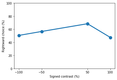
As expected on the first day of training the mouse has not yet grasped the concept of the task and performed at chance level. We can break down the performance at each contrast level and create a simple plot. In this plot let’s also express performance in terms of rightward choice.
[19]:
import matplotlib.pyplot as plt

contrast_performance = np.empty((contrasts.size))
for ic, c in enumerate(contrasts):
    contrast_idx = np.where(trials_day1.contrast == c)[0]
    if c < 0:
        contrast_performance[ic] = 1 - (np.sum(trials_day1.feedbackType
                                               [contrast_idx] == 1) / contrast_idx.shape[0])
    else:
        contrast_performance[ic] = (np.sum(trials_day1.feedbackType
                                           [contrast_idx] == 1) / contrast_idx.shape[0])

plt.plot(contrasts * 100, contrast_performance * 100, 'o-', lw=3, ms=10)
plt.ylim([0, 100])
plt.xticks([*(contrasts * 100)])
plt.xlabel('Signed contrast (%)')
plt.ylabel('Rightward choice (%)')

print(contrast_performance)
[0.50617284 0.56666667 0.68493151 0.475 ]
As the mice learns the task we expect its performance to improve. Let’s repeat the steps above and see how the same mouse performed on day 15 of training
[20]:
eid_day15 = eids[14]
trials_day15 = one.load_object(eid_day15, 'trials')
n_trials_day15 = len(trials_day15.choice)

trials_day15.contrast = np.empty((n_trials_day15))
contrastRight_idx = np.where(~np.isnan(trials_day15.contrastRight))[0]
contrastLeft_idx = np.where(~np.isnan(trials_day15.contrastLeft))[0]

trials_day15.contrast[contrastRight_idx] = trials_day15.contrastRight[contrastRight_idx]
trials_day15.contrast[contrastLeft_idx] = -1 * trials_day15.contrastLeft[contrastLeft_idx]

contrasts, n_contrasts = np.unique(trials_day15.contrast, return_counts=True)
print(f"Visual stimulus contrasts on day 15 = {contrasts * 100}")
print(f"No. of each contrast on day 15 = {n_contrasts}")
local md5 or size mismatch, re-downloading C:\Users\Mayo\Downloads\FlatIron\cortexlab\Subjects\KS022\2019-10-15\001\alf\_ibl_trials.included.npy
100%|████████████████████████████████████████████████████████████████████████████| 648/648 [00:00<00:00, 107308.47it/s]
Downloading: C:\Users\Mayo\Downloads\FlatIron\cortexlab\Subjects\KS022\2019-10-15\001\alf\_ibl_trials.included.c98b22fc-5c11-481b-b7cb-8b5f3a90f105.npy Bytes: 648
Visual stimulus contrasts on day 15 = [-100.   -50.   -25.   -12.5   12.5   25.    50.   100. ]
No. of each contrast on day 15 = [ 94  65 107  16  21  75  78  64]
Notice how on day 15 the mouse not only has trials with 100 % and 50 % visual stimulus contrast but also 25 % and 12.5 %. This follows the IBL training protocol where harder contrasts are introduced as the mouse becomes more expert at the task.
[21]:
correct = np.sum(trials_day15.feedbackType == 1) / n_trials_day15
print(f"Correct = {correct * 100} %")
Correct = 88.26923076923077 %
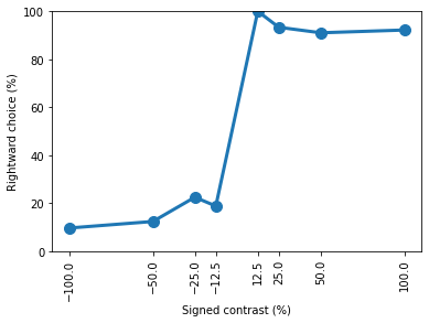
The performance has vastly improved compared to day 1 of training! Once again let’s break this down further into the performance at each contrast and create a plot of rightward choice vs signed contrast
[22]:
contrast_performance = np.empty((contrasts.size))
for ic, c in enumerate(contrasts):
    contrast_idx = np.where(trials_day15.contrast == c)[0]
    if c < 0:
        contrast_performance[ic] = 1 - (np.sum(trials_day15.feedbackType
                                               [contrast_idx] == 1) / contrast_idx.shape[0])
    else:
        contrast_performance[ic] = (np.sum(trials_day15.feedbackType
                                           [contrast_idx] == 1) / contrast_idx.shape[0])

plt.plot(contrasts * 100, contrast_performance * 100, 'o-', lw=3, ms=10)
plt.ylim([0, 100])
plt.xticks([*(contrasts * 100)])
plt.xlabel('Signed contrast (%)')
plt.ylabel('Rightward choice (%)')
plt.xticks(rotation=90)

print(contrast_performance)
[0.09574468 0.12307692 0.22429907 0.1875     1.         0.93333333
 0.91025641 0.921875  ]
You should now be familiar with the basics of how to search for and load data using ONE and how to do some simple analysis with data from the IBL task. To see how to replicate this tutorial using Datajoint, please see this tutorial.