Exploring the public IBL data with ONE
This tutorial will give an introduction into the publically available data and show how to download electrophysiology data for a probe insertion and display a simple raster plot
First let’s get started by importing the ONE module and connecting to the database
[1]:
# Import one and connect to the database
from one.api import ONE
one = ONE(base_url='https://openalyx.internationalbrainlab.org', silent=True)
We want to see what probe insertions are available on the database. To list them we can use the following command
[2]:
probe_insertions = one.alyx.rest('insertions', 'list')
We can find the number of probes insertions available and some information about the first probe
[3]:
from pprint import pprint
print(f'N probes = {len(probe_insertions)}')
pprint(probe_insertions[0])
N probes = 4
{'auto_datetime': '2021-04-02T15:03:46.367818',
 'datasets': ['8091108f-a0d2-44e0-bf01-5c0a93de7844',
              '54e5d55d-e19d-452d-beed-ff49a5b3b38b',
              'eaed8cf5-0bb9-4eaf-8d8e-3471e39d63fa',
              '236a116c-8a18-4dd0-a2b5-169b28ef7fd4',
              'a3bf84f1-3ee2-4f3c-a36a-4b4959a513ba',
              'bce68e1c-1d72-4bf9-b77f-0c9e3b1c5c12',
              'c0c3c1a7-ee4d-4117-8a6f-93d9d43c52ee',
              'e9d8ddb5-ddaf-48b7-8a78-49d909c80ef1',
              '138676a2-d310-49b4-865e-0e14f8b13182',
              '837af07a-26aa-4264-97d6-fa55d2382f77',
              '4f397701-da2e-460b-9937-a6a53ff23959',
              '45854a1c-c309-4bb0-806e-a4f9f1617472',
              'b31f4721-0163-4aec-a92e-7353764ce355',
              '25c2b0f4-6201-407d-8cf6-f892370a5a44',
              'ffea1a62-dc7e-4d01-8f86-03801a88615f',
              'eaa07c05-df66-42ce-ae59-326b6ac9e8f0',
              '4420d325-141b-4d30-8b92-0f8f545274d3',
              '6a0c68d2-2728-4d3d-8422-2228fe52226b',
              '99c957a8-f664-463b-afae-a1ba570a85b2',
              '94285bfd-7500-4583-83b1-906c420cc667',
              '5c814a9b-be69-4513-8282-a8fd3d562521',
              '40af4a49-1b9d-45ec-b443-a151c010ea3c',
              'ea257f30-8a0f-4cde-83d2-aa4d2ce4bd23',
              'dd78976c-fc95-4221-83db-a034652b8867',
              '3d9cbd53-fe3f-41ca-ae37-71936f5ca68f',
              '3d1fc6f0-48bc-493e-834d-d1cf6a496255',
              '854e2ec7-c974-4dcc-8dea-b0a6063febdf',
              '322e85c0-b5d8-4013-9db0-5f523a2a489c',
              '600b333b-030b-482f-a02f-0a8b90e73eab',
              'a51473f0-4139-4d01-9264-bea36db1789a',
              'cf745deb-4a45-418f-9871-6a51a6ec712d',
              '582cd4c3-02b8-4121-84ba-f4611aa4dcfe',
              '249fd743-3207-478f-923a-45749d92d87b',
              '7fbebff5-8f6a-4b4b-aeba-c5a9118343db',
              '545f7a74-9a47-438b-8367-d715d70a3710',
              '5327c66d-dab0-41b3-b180-3aa7d47d5303',
              'af8dd0e9-2057-4d2c-b47f-2598153f187d',
              '6cd3b0c3-8d83-4367-b554-f90f8d505c0e',
              '0d0bad29-7f05-4825-8cf9-50d9b7dc83c3',
              'cc9bf356-9ec2-4100-8256-4a0363d2085a',
              '9314c967-4b92-421a-8956-3daaf5be1da7',
              '00c234a3-a4ff-4f97-a522-939d15528a45',
              '53ab50fe-b57d-4013-909f-05219e77b053',
              '10ee20c5-71dc-4e6d-9c52-45c78d9ac57b'],
 'id': 'da8dfec1-d265-44e8-84ce-6ae9c109b8bd',
 'json': {'amplitude_max_uV': 927.98,
          'amplitude_median_uV': 637.25,
          'drift_rms_um': 2.53,
          'extended_qc': {'alignment_count': 1,
                          'alignment_resolved': False,
                          'alignment_stored': '2021-04-02T15:03:41_nate',
                          'experimenter': 'PASS',
                          'tracing_exists': True},
          'firing_rate_max': 72.82,
          'firing_rate_median': 3.95,
          'n_units': 794,
          'n_units_qc_pass': 280,
          'qc': 'PASS',
          'whitening_matrix_conditioning': 11.66,
          'xyz_picks': [[786, 624, -568],
                        [786, 624, -767],
                        [761, 624, -942],
                        [710, 599, -1068],
                        [611, 599, -1218],
                        [511, 550, -1468],
                        [386, 550, -1718],
                        [211, 524, -2093],
                        [11, 499, -2668],
                        [-88, 474, -2918],
                        [-88, 474, -3093],
                        [-139, 449, -3243],
                        [-413, 425, -3993],
                        [-488, 425, -4242],
                        [-563, 400, -4468],
                        [-813, 400, -5267],
                        [-913, 324, -5743],
                        [-938, 324, -5893],
                        [-938, 324, -6117]]},
 'model': '3B2',
 'name': 'probe00',
 'serial': '19108320031',
 'session': '4ecb5d24-f5cc-402c-be28-9d0f7cb14b3a',
 'session_info': {'id': '4ecb5d24-f5cc-402c-be28-9d0f7cb14b3a',
                  'lab': 'hoferlab',
                  'number': 1,
                  'start_time': '2020-09-21T19:02:16.707541',
                  'subject': 'SWC_043',
                  'task_protocol': '_iblrig_tasks_ephysChoiceWorld6.4.2'}}
Each probe insertion has a unique ID (pid) that we can use to search the database and find the datasets that are linked to it. Let’s look at the datasets associated with the first probe in the list
[4]:
pid = probe_insertions[0]['id']

datasets = one.alyx.rest('datasets', 'list', probe_insertion=pid)
print(f'N datasets = {len(datasets)}')
pprint(datasets[0])
N datasets = 44
{'auto_datetime': '2021-02-10T20:24:31.484939',
 'collection': 'alf/probe00',
 'created_by': 'afb0fdad',
 'created_datetime': '2020-09-22T09:31:52.393857',
 'data_format': 'csv',
 'dataset_type': 'clusters.uuids',
 'default_dataset': True,
 'experiment_number': 1,
 'file_records': [{'data_repository': 'flatiron_hoferlab',
                   'data_repository_path': '/public/hoferlab/Subjects/',
                   'data_url': 'https://ibl.flatironinstitute.org/public/hoferlab/Subjects/SWC_043/2020-09-21/001/alf/probe00/clusters.uuids.3d9cbd53-fe3f-41ca-ae37-71936f5ca68f.csv',
                   'exists': True,
                   'id': 'ae3974e1-7cdc-42cb-8632-b9ae0391e71d',
                   'relative_path': 'SWC_043/2020-09-21/001/alf/probe00/clusters.uuids.csv'}],
 'file_size': 29383,
 'hash': '41ec5a83b7d7f41df9730fcae9cc7024',
 'name': 'clusters.uuids.csv',
 'protected': False,
 'public': False,
 'revision': None,
 'session': 'https://openalyx.internationalbrainlab.org/sessions/4ecb5d24-f5cc-402c-be28-9d0f7cb14b3a',
 'tags': [],
 'url': 'https://openalyx.internationalbrainlab.org/datasets/3d9cbd53-fe3f-41ca-ae37-71936f5ca68f',
 'version': '1.5.36'}
To get a more concise summary of the datasets available we can loop through and display their names
[5]:
dataset_names = [dset['name'] for dset in datasets]
pprint(dataset_names)
['clusters.uuids.csv',
 'spikes.clusters.npy',
 'spikes.times.npy',
 'spikes.samples.npy',
 '_kilosort_raw.output.tar',
 'clusters.amps.npy',
 '_spikeglx_sync.channels.probe00.npy',
 '_spikeglx_sync.times.probe00.npy',
 'spikes.amps.npy',
 'clusters.metrics.pqt',
 'clusters.waveformsChannels.npy',
 'clusters.waveforms.npy',
 'clusters.peakToTrough.npy',
 'channels.rawInd.npy',
 '_spikeglx_sync.polarities.probe00.npy',
 'clusters.depths.npy',
 'spikes.depths.npy',
 'clusters.channels.npy',
 '_spikeglx_ephysData_g0_t0.imec0.ap.cbin',
 '_spikeglx_ephysData_g0_t0.imec0.lf.cbin',
 '_spikeglx_ephysData_g0_t0.imec0.lf.ch',
 '_spikeglx_ephysData_g0_t0.imec0.ap.ch',
 '_spikeglx_ephysData_g0_t0.imec0.ap.meta',
 '_spikeglx_ephysData_g0_t0.imec0.lf.meta',
 '_spikeglx_ephysData_g0_t0.imec0.sync.npy',
 '_spikeglx_ephysData_g0_t0.imec0.timestamps.npy',
 '_spikeglx_ephysData_g0_t0.imec0.wiring.json',
 'spikes.templates.npy',
 'channels.localCoordinates.npy',
 'templates.waveformsChannels.npy',
 'templates.waveforms.npy',
 'templates.amps.npy',
 '_iblqc_ephysTimeRmsLF.timestamps.npy',
 '_iblqc_ephysTimeRmsAP.timestamps.npy',
 '_iblqc_ephysTimeRmsLF.rms.npy',
 '_iblqc_ephysTimeRmsAP.rms.npy',
 '_iblqc_ephysSpectralDensityLF.freqs.npy',
 '_iblqc_ephysSpectralDensityAP.freqs.npy',
 '_iblqc_ephysSpectralDensityLF.power.npy',
 '_iblqc_ephysSpectralDensityAP.power.npy',
 '_kilosort_whitening.matrix.npy',
 '_phy_spikes_subset.channels.npy',
 '_phy_spikes_subset.spikes.npy',
 '_phy_spikes_subset.waveforms.npy']
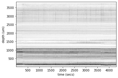
We are interested in downloading the spikes datasets output from spike sorting in order to display a raster plot of the neural activity recorded on the probe. To download the data we can use the following approach
[6]:
dtypes = ['spikes.times',
          'spikes.depths',
          'spikes.amps']
eid, probe = one.pid2eid(pid)
spikes = one.load_object(eid, 'spikes', collection=f'alf/{probe_insertions[0]["name"]}',attribute=['times', 'depths',
                                                                                                   'amps'])
We can import a module from brainbox that plots the raster across time
[7]:
from brainbox.plot import driftmap
driftmap(spikes['times'], spikes['depths'], t_bin=0.1, d_bin=5)
Out[7]:
<AxesSubplot:xlabel='time (secs)', ylabel='depth (um)'>